TUTORIAL
Introduction
The purpose of this tutorial is to familiarise you as quickly as possible with the main features of the Proteus layout module to the point that you can use the package for real work. Users with modest computer literacy should find it possible to learn the package and produce their first board within a day or two.
The tutorial proceeds by taking you through worked examples involving all the important aspects of the package including:
- Basic techniques for placement and routing.
- 3D board visualisation.
- Netlist based design including both manual and automatic routing.
- More advanced editing techniques such as block editing and route editing.
- Hard copy and managed manufacturing output.
- Library part creation.
We do urge you to work right the way through the tutorial exercises as many things are pointed out that if missed will result in much wasted time in the long run. Also, having worked through the tutorial and thus got a basic grasp of the concepts behind the package you will find it much easier to absorb the material presented in the reference chapters.
Note that throughout this tutorial (and the documentation as a whole) reference is made to keyboard shortcuts as a method of executing specific commands. The shortcuts specified are the default or system keyboard accelerators as provided when the software is shipped to you. Please be aware that if you have configured your own keyboard accelerators the shortcuts mentioned may not be valid. You can configure your own keyboard shortcuts via the System - Set Keyboard Mapping command.
Menus toolbars and icons all switch when you change between tabs to reflect the functionality of the module you are working on. When we talk about menu commands or icons in this tutorial we assume that the PCB layout tab is selected. The menu contents will be very different if the schematic tab is selected!
See Also:
Application Framework : Backup and Recovery Procedures
Overview of the Layout Editor
We shall assume at this point that you have installed the package, and that the current directory is some convenient work area on your hard disk. This tutorial is a direct continuation of project we started in the schematic capture tutorial so we will start by loading the project file with the completed schematic.
From the home page in Proteus click on the Open Sample button, filter to the tutorials category and then select the dsPIC33 Recorder (schematic only) sample.
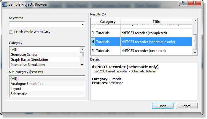
Opening a Tutorial sample design
This will open the tutorial project with the completed schematic from the schematic capture tutorial. We can start the PCB layout module from the application module toolbar at the top of the Proteus application.
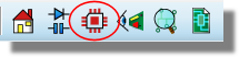
If you are working on two monitors or have free screen space you can drag and drop one of the tabs to view both modules simultaneously. If not, you can switch between the tabs with the mouse or via the standard windows CTRL+TAB shortcut key.
Much of the look and feel of the application is similar to the Proteus capture module and hopefully now familiar, although there are some important differences.
The Main Window
The largest area of the screen is called the Editing Window, and it acts as a window on the drawing - this is where you will place and track the board. The smaller area at the top left of the screen is called the Overview Window. In normal use the Overview Window displays, as its name suggests, an overview of the entire drawing - the blue box shows the edge of the current sheet and the green box the area of the sheet currently displayed in the Editing Window. However, when a new object is selected from the Object Selector the Overview Window is used to preview the selected object - this is discussed later.
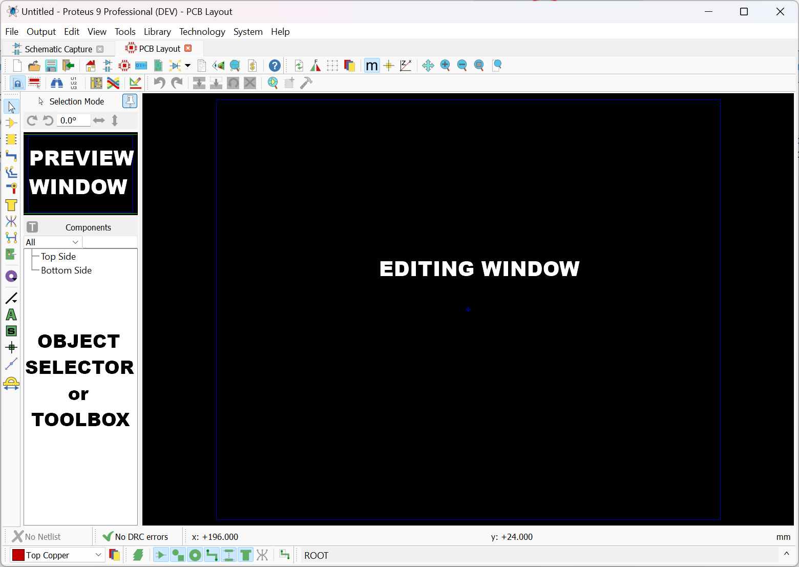
PCB Layout Editor Window
See Also:
Screen Layout (Reference Manual)
Toolbars
There are icon toolbars for command sets (along the top) and modes of operation (down the side). You can turn toolbars on and off from the toolbars command on the View Menu. However, it is perhaps more useful to collapse toolbar groups that are used infrequently.
To collapse a toolbar group right click on one of the icons and select the collapse command from the resulting context menu.
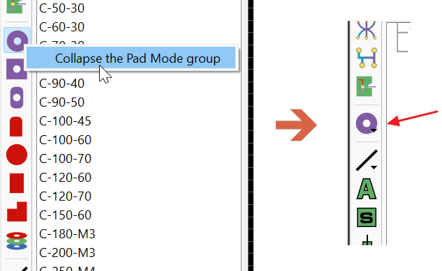
Collapsing the pad modes toolbar group
To select an icon in a collapsed group (switch modes) right click on the group and then select the mode you want from the resulting context menu.
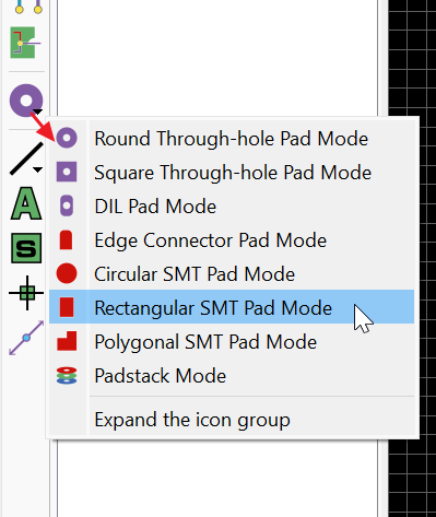
Switching to a different pad mode in a collapsed toolbar group
To expand a collapsed toolbar group right click on the group and select the expand option at the bottom of the resulting context menu.
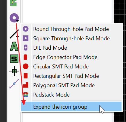
Expanding the pad modes toolbar group
Depending on your monitor and your preferences you might find that using collapsed toolbar groups together with larger icons provides more clarity without consuming lots of editor space.
The Control Bar
The control bar at the bottom of the application is different from what we have seen in the schematic capture module and essentially splits into five sections:
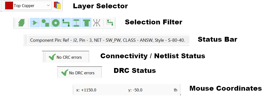
The control bar, showing the selection filter, the layer selector and the layer visibility icon on the left, the status bar in the middle, and the connectivity, DRC and co-ordinate readouts on the right
At the left hand side is the Selection Filter which allows you to configure both the layers and the objects that will be selected in the current operating mode. Typically, the default rules will suffice and this serves simply as a convenient override where you may wish finer granularity in selection at a given time. The Layer Selector combo box also determines the current layer or layer set and also applies to the placement of PCB objects.

The Layer and Selection filter
In the middle is the Status Bar which provides textual ‘hints’ on the object currently under the mouse. This is particularly useful when you hover a mouse over a pad for example, as it will inform you which net the pad is on.
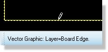
The Status bar shows what the mouse is pointing at
The status bar is also particularly helpful when placing or editing tracks, providing information about the current routing mode as well as net and route length information.

Routing information on the status bar as track is being placed.
Next, we have the connectivity status which controls the syncing of the PCB to the schematic and - when everything is synchronised - doubles as a live connectivity checker.

Netlist Information and CRC information on the status bar
Next to the connectivity status is the live Design Rule Checker. This will report any physical design rule violations that occur while the board is being designed. A left click on this will launch a dialogue detailing the violations with the further option of zooming in to examine a particular error.

DRC information on the status bar
Finally, at the far right hand side is the co-ordinate display which reads out the position of the cursor when appropriate. These reflect not the exact position of the pointer but the location to which it has been snapped. Default snapping options are selectable from the View menu (or via keys CTRL+F1 and F2 to F4) and the snap values can be configured from the Set Grid Snaps command on the Technology menu.

Mouse Co-ordinates
The co-ordinates can be in imperial or metric units as set by the Metric (default key mapping 'M') command. You can also set a false origin using the Origin command (default key mapping 'O') in which case the co-ordinates change colour from black to magenta.
The dot grid on the Editing Window can be toggled on and off using the Grid command, or via it’s keyboard shortcut (by default this is ‘G’). The spacing of the dots normally reflects the current snap setting, except when zoomed out. In this case, the dot spacing is set to a suitable multiple of the snap spacing.
An X cursor can be displayed at the position to which it has snapped the pointer through the X-Cursor command, default key mapping is 'X'.
We’ll become familiar with all of these items and use them regularly as we work through placement and routing of the board.
See Also:
Selection Filter (Reference Manual)
Navigation
Navigation of the layout (middle mouse zoom, panning, keyboard shortcuts, etc.), is identical to the schematic capture package. Refer to the Schematic Capture Getting Started Guide or the Schematic Reference Manual for more information.
Visual Aids to Design
As in the capture module, Proteus PCB layout will use visual effects to help you understand what is happening during board layout. There are two principle techniques:
- Proteus will ‘twitch’ an object when that object is under the mouse and the selection filter enables selection of that object type. This serves to identify when an object is ‘hot’.
- Dynamic cursors are provided which change to identify what a left click will do at any given time (place an object, select an object, move an object, etc.). A list of cursor types is shown below.
| Cursor | Description |
|
|
Standard Cursor |
|
|
Placement Cursor - Left click will place and object according to mode. |
|
|
Selection Cursor - left click will select the object under the mouse. |
|
|
Movement Cursor - left drag will move the object selected. |
|
|
Push Limit Cursor - indicates that the current push operation (either in route placement or route editing) has reached limit of possible objects. If this happens unexpectedly it's most often because vias have been pushed causing tracks on other layers to also be pushed resulting in a cascade effect. |
|
|
No Entry Cursor - indicates that the current route placement or editing operation has hit an obstacle and moving further would result in a design rule error. With long tracks this can happen outside of the current viewable area and with push routing it can happen on other layers if you push vias. |


Visual DRC
Visual DRC provides a viewport around the mouse and each object shows an expansion corresponding to it's design rule clearance in an overlay. This instantly lets you see whether the route being placed/edited can move where you want it to go and then take action such as toggling push mode or changing track style to squeeze through a tight gap.
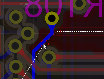
Visual DRC Auras around Tracks and Vias when placing a route.
Visual DRC is on by default but can be toggled with the SHIFT+D keyboard shortcut and can be configured via the Route Command Centre (keyboard 'R').
See Also:
Throughout this tutorial – and indeed whenever you are working in Proteus – you should make use of these visual indicators to as an aid to understanding the software.
Proteus includes a multi-level ‘undo’ and ‘redo’ system via the shortcut keys CTRL+Z and CTRL+Y respectively. If you make mistakes throughout the tutorial remember that you can unwind as many times as you need to!
Themes & Icons
Proteus supports both a standard (light) and a dark mode theme. You can switch between themes and set icon sizes from the System Menu - System Settings command.
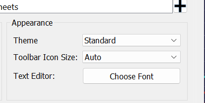
A Proteus restart is required for changes to take effect.
Display Options
Proteus is capable of harnessing the power of your computers graphics card to speed up operation and provide true layer transparency on the layout. However, as not all machines have sufficient graphics cards the software is also capable of using Windows to perform display and graphical operations. Four modes of operation are offered:
- Use Windows GDI Graphics.
- Use Software Graphics.
- Use Open GL Graphics (Hardware Accelerated).
- Use Direct2D Graphics (Hardware Accelerated).
Proteus will test your computer when you first open the application and, if possible, will then set a default hardware accelerated mode for you. Control over hardware acceleration and display options can be found via the Set Display Options command on the System Menu. Some options are relevant only to a particular mode and will be disabled if you select a different mode.
Graphics Mode
The first section of the dialogue reports on whether your graphics card will support OpenGL or Direct2D hardware acceleration and, if so, allows you to switch from Windows GDI mode into one of these two modes.
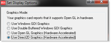
Select the best option that your graphics card supports.
Opacity
When a hardware accelerated display mode is selected the Opacity section of the dialogue allows you to configure the transparency of various layers on the board.
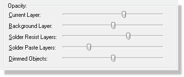
Opacity options
When using hardware acceleration, Proteus places special significance on the current layer, giving it a higher opacity than other copper layers on the layout. This means that objects on the layer you are working are clearly visible and that objects on the other layers of the board are dimmed. You can control the relative opacity of both the current layer and the background layer(s) using the sliders on this section of the dialogue form. For example, if you wish to disable transparency altogether you could set the background layer slider to maximum.
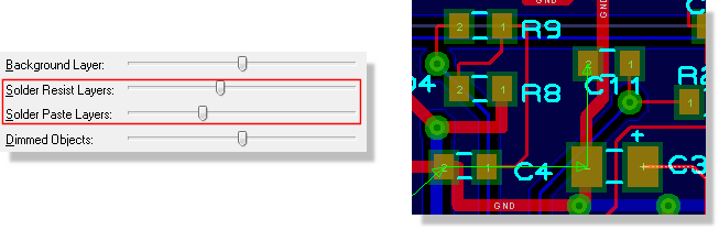
Additionally, with hardware acceleration you can live view the solder resist and paste mask around pads and vias on the layout (turn on/off from View Menu - Layers). When enabled, you can also adjust the opacity of these layers using the appropriate slider controls
If you are working on complex, multi-layer PCBs it can be useful to define a number of preset views for the board. This is done by creating new colour sets in the displayed layers dialogue (e.g. TOP_VIEW, BOT_VIEW) with appropriate layers visible and assigning them keyboard shortcuts.
See Also:
Auto-Pan Animation
In Proteus, holding down the shift key and bumping the mouse against the edge of the Editing Window allows you to pan the screen. Similarly, dragging an object against the edge of the Editing Window will pan the screen in the direction of the drag. This navigation feature is called auto-pan and is controlled via the options in this section of the dialogue form.
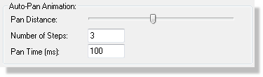
Auto-Pan options
You can adjust the distance moved on auto-pan (pan distance), the number of steps taken to cover this distance (number of steps) and the speed of the animation (pan time). These options are available regardless of which mode of operation you have specified.
Highlight Animation
When working in hardware accelerated mode objects under the mouse with smoothly increase their intensity to inform you that they are selectable. The highlight animation options on this dialogue allows you to control the smoothness and speed of this effect.
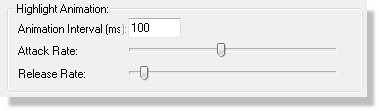
Animation Speed options
The animation interval controls the frame rate of the animation and therefore the smoothness of the fade-in/fade-out effect. Normally, the default value for this is suitable.
The attack rate specifies the speed at which an object will go from ‘fully off’ to ‘fully on’ whilst the release rate allows you to adjust the speed at which an object will return from ‘fully on’ to ‘fully off’.
These options are only available in hardware accelerated modes.
Multi-Sampling (Anti-Aliasing)
Multi-Sampling is a method used by graphics cards to reduce anti-aliasing effects when graphics are displayed at different zoom levels. It is particularly applicable to text but impacts on all graphics on the layout.

When working in OpenGL mode you can specify the level of multi-sampling you want to use. The higher the level of multi-sampling the better the resulting display but the more GPU resources are consumed. If you select a level of multi-sampling which is not supported by your graphics hardware the software will reset the level to the closest one which your card can handle. For normal operation in Proteus a multi-sampling level of 4x is quite sufficient.
Displayed Layers Dialogue
The displayed layers dialogue allows you to control the visibility and colour of the various layers on the board. You can launch this from the View menu or by clicking the mouse layers icon at the bottom of the application.
You can change the colour of a layer by clicking on the colour beside the layer and control the visibility of the layer via the checkbox beside the layer (where appropriate). All changes are updated live on the layout.
You can switch between the pre-supplied colour profiles (print and screen), create your own colour profiles via the 'new' button at the top of the dialogue form and assign them to keyboard shortcuts. This allows you for example to have a TOP colourset showing only top copper, top silk, top resist and top paste mask. Adding a colour set for TOP ASSEMBLY for example is also quite common. More information is available via the context sensitive help for the dialogue form (click on the question mark at the top right of a dialogue and then on a field of the dialogue form to launch).
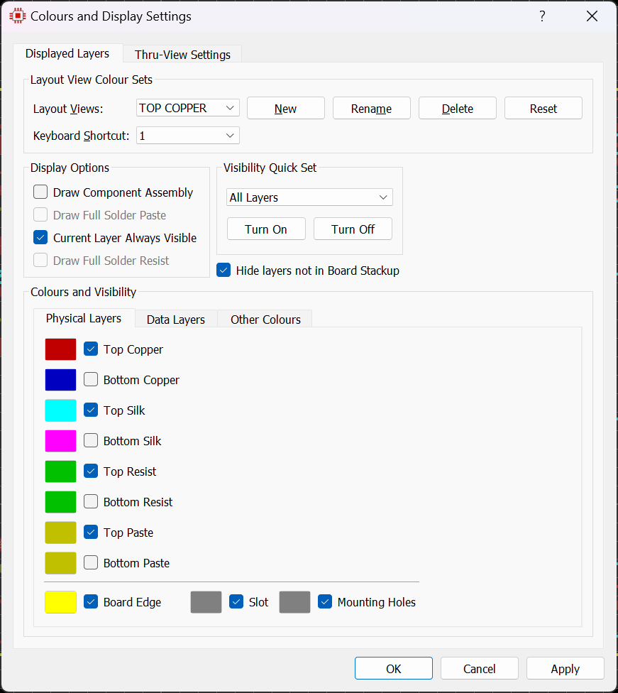
Displayer Layers form with Top layers only selected
Finally, if you are working in OpenGL or Direct2D mode, the Resist/Paste Mask Display options allow you turn on full display of these layers on the board, showing the resist and paste coverage around pads and vias. When enabled you can change the intensity of these layers by switching to the Thru-View settings tab and adjusting the appropriate slider controls.
Component Placement
Proteus works with a live netlist so the layout module already has much of the information we need to start the layout process. In particular, we have specified which footprints are associated with each schematic symbol and so Proteus can therefore pre-select these for us ready for placement. This brings us to an important distinction in the software; the difference between a component and a package.
Components and Packages
- A component is an instance of a footprint that has been netlisted through from the schematic.
- A package is a physical footprint that exists in the PCB Layout Libraries.
More information on the Libraries can be found here
Selecting component mode will access footprints which have been specified as relating to parts in the associated schematic and carry connectivity information whereas selecting package mode will access ‘unbound’ physical instances of a footprint. When working with a layout which is driven from a schematic we therefore exclusively use component mode.
The Component Mode icon is second from the top directly underneath the Selection icon. Clicking on this will display a list of items in the Object Selector which correspond directly to the parts on the schematic.
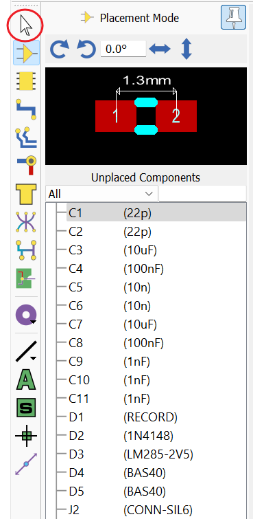
Component Mode
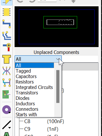
The combo box at the top of the component list allows you to filter the list into a smaller set to help you organise the order in which you place parts on the board. Common filters include:
- Tagged : Allows you to select a section of schematic and then see those footprints. Enables board layout in logical blocks.
- Group Name : If you set up named groups for components then you can filter to place by group. This is discussed in more detail in Autoplacement section of the main reference manual.
The Package Mode icon is directly underneath the Component mode icon and clicking on this will show us the physical footprints corresponding to the components in the layout.
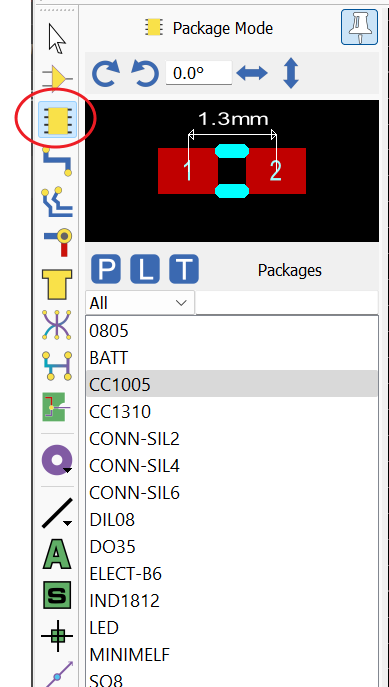
Package Mode
Note that you can right click on any package to tag all instances of the package currently on the board.
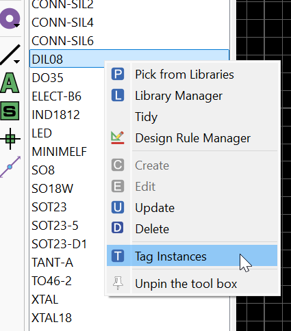
When placing, routing and laying out a PCB based on a schematic (such as with this project) we will be working with components.
The Board Edge
Before we can place the components on the board we need to define what shape and size the board will be. For our project we need only a simple rectangular board edge but we do want to control the dimensions of the board (115mm wide and 40mm high).
The first thing to point out here is that the layout module will operate in either imperial or metric units and you can switch between modes either by toggling the Metric command on the View menu or via the ‘M’ keyboard shortcut. You may need to switch units for the placement of the board edge and also elsewhere in the documentation.
You can set your default or preferred units from Technology Menu - Set Grid Snaps command.
To start placing the board edge, select the 2D Rectangle icon from the left hand side of the application.

2D Box Icon
Next, change the Layer Selector to the Board Edge Layer.

Board Edge layer selected
Move the mouse to the approximate starting point (e.g. top left) for the board edge. Now, hold the mouse still and press the ‘O’ key on the keyboard to set the origin of the co-ordinate system to the point under the mouse. This will be reflected in the co-ordinate display at the bottom right of the application. Left click to start placement and drag in the normal way. The co-ordinate display at the bottom will show you the dimensions of the board edge as you drag.
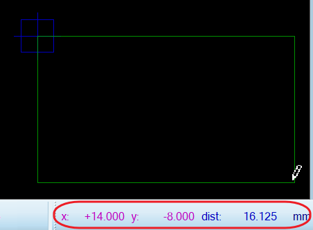
Drawing a board edge
Press the ‘M’ key on the keyboard to toggle between metric and imperial units as required. Once you have the desired size of board edge click left again to commit placement. Don’t worry about where in the Editing Window you have placed the board edge – we will move it to the centre of the world area shortly.
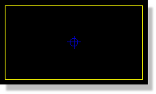
Placed board edge which is always Yellow
If you would like the board edge to be a specific size, Edit the board edge graphic and set the dimensions to your requirements:
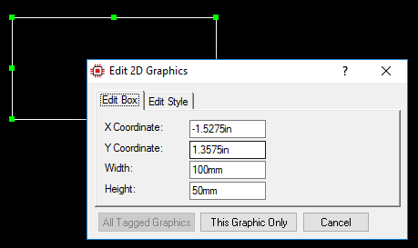
Setting the dimensions of the board edge
Finally, restore the co-ordinate system to it’s global origin by pressing the ‘O’ button on the keyboard again. The colour of the co-ordinates will change from Magenta to black to indicate that the global origin is now in use.

Co-ordinates at 0,0
Placing a board edge should always be the first task as the software needs to know the boundaries of the board in order for example, to know the limits of where the autorouter can function or the size of a power plane.
If you need to delete the board edge or resize it, you can do so via the context menu options and drag handles that will appear when you right click over the board edge graphic.
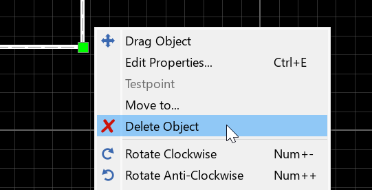
Select Delete from the context menu
Board Edges of any complexity are best brought in from the MCAD tool via the Import DXF command on the File Menu (and placed onto the board edge layer ! )
Vertices / Nodes & Handles
It is well known that not all board edges are a simple rectangle. If you need your own shape, you can use the 2D Path Tool to draw more complex shapes. Holding the CTRL key down will allow you to draw a curve. Once the main shape is completed (Start and end on the same grid point), you can edit it to make finer adjustments:
- ALT + Left click will allow you to add nodes / vertices
- ALT + Right click will allow you to delete nodes / vertices
See Also:
Layer Stackup and Drill Spans
Before we begin layout, we need to define our layer stackup and specify which drill ranges are valid for vias. Start by launching the Set Layer Stackup command from the Technology menu.
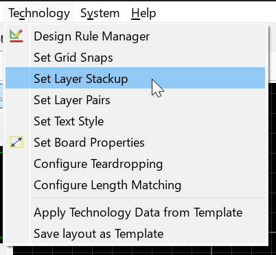
The Set Layer Stackup command on the Technology menu
We will be making a simple two-layer board with a single core between top copper and bottom copper. This will be shown visually on the editable grid and as a cross section in the board view tab.
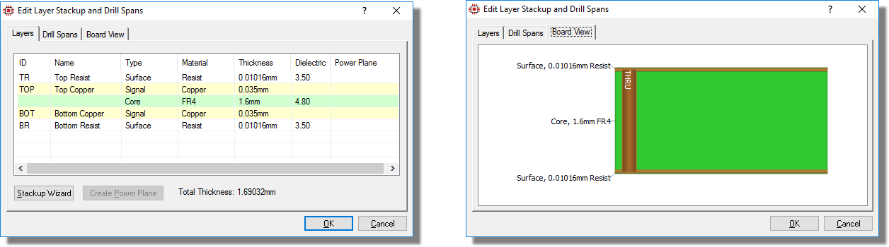
The default two layer stackup on the Layers tab, and the same stack drawn as a cross section on the Board View tab
Since the defaults are fine for us, there is no action required here. If we did want to edit the stackup then we would do so via the stackup wizard button which would allow us to change the number of copper layers and the construction method for the board. The construction method is chosen from the Board Style dropdown, which offers Internal Layers, External Layers and 1+n+1 HDI (single buildup).
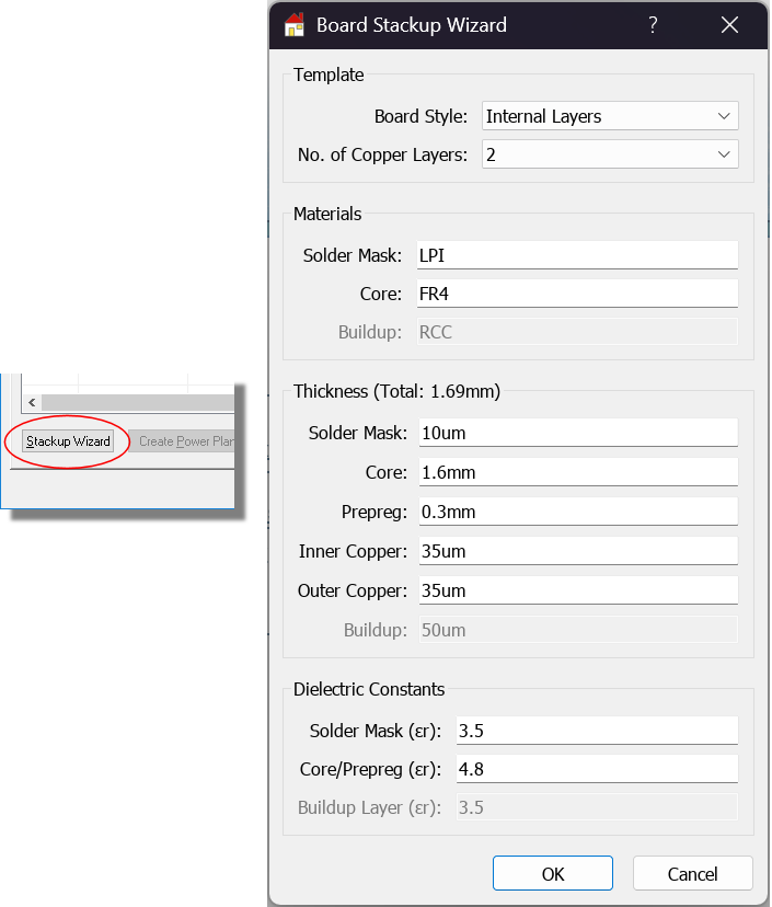
The Stackup Wizard button and the Board Stackup Wizard dialogue form it launches
Similarly, on the drill spans tab there are no additions required, since our target PCB is 2-layer only. However, to provide some context to the topic, the following are some screenshots from a 6-layer stackup.
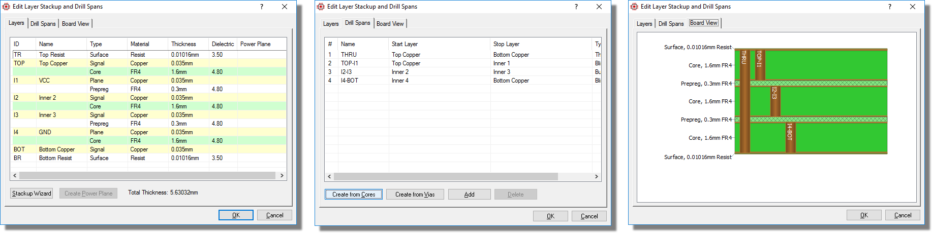
A six layer stackup, showing the layers, the drill spans defined for them and the resulting board cross section
The most important thing to remember is that for multi-layer boards, configuration of this dialogue is really important. The stack distinguishes mechanically drilled spans from laser-drilled micro-via spans, so the drill spans you define here are what tell Proteus which vias are physically possible on your board. The setting up of the drill ranges enables the use of smart vias which use the smallest drill range that will switch between routing layers. This is very powerful and convenient when placing tracks across layers so a little time spent here can save a lot of time later in the layout process. We'd encourage you to read through the dialogue level help and if you are unsure about anything, the topic is discussed in detail in the reference manual.
The question mark button at the top right of the dialogue launches its context sensitive help
If you are designing high density boards, the stackup wizard also offers a 1+n+1 HDI board style. This creates a single buildup layer construction with micro-via drill spans on the outer layers, suitable for designs that use laser-drilled micro-vias. HDI templates are also available from the New Project wizard for common configurations such as 4-layer (1+2+1), 6-layer (1+4+1) and 8-layer (1+6+1).
See Also:
Reference Manual : About Layer Stacks
Reference Manual - About Drill Spans
Reference Manual - 1+n+1 HDI Construction
Reference Manual - Specifying Plane Layers
Work Area, Co-ordinates and Snap
It is likely that your board edge covers a small portion of the Editing Window, which is less than ideal as all of the work will be taking place inside this area. We can of course zoom into the area (point the mouse and roll the middle mouse button or use the F6 key) but the default zoom level is designed to show the entire Work area. The Work area is the area inside the dark blue box at the edges of the Editing Window. Let’s tidy this up a bit before we move on.
Start by switching into Selection Mode and then left click and drag a selection box around the board edge.
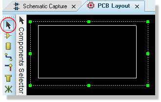
Selection mode and the board edge selected
If you get it wrong and don’t completely cover the board edge, use the green handles to resize the selection box until it completely encompasses the board edge.
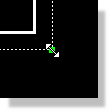
Resizing a box by the drag handles
Now place the mouse inside the selection box, depress the left mouse button and drag into the centre of the work area, releasing the mouse button to commit the placement.
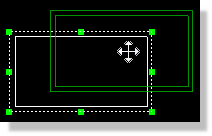
Moving the board edge
This is a very important technique worth mastering as it allows you to easily block select and then perform actions on (move, delete, etc.) groups of objects.
A selection box is temporary; it lasts only until you click elsewhere. For clusters of objects that you expect to move together repeatedly, Proteus can make the association permanent with an object group. We will do exactly that when we come to place the mounting holes.
Having centred our board edge in the Work area we can shrink the work area to a suitable size. From the Technology Menu, select the Set Board Properties command and then set to something like 175mm by 100mm, such that the resulting work area forms a reasonable boundary to the board.
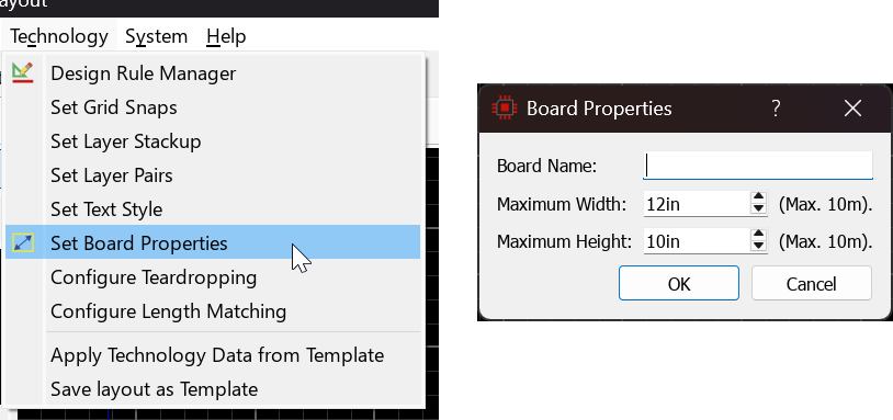
Setting the board properties
We saw briefly when placing the board edge that we can specify a temporary origin and use that to place items of a given size (or to place items a specific distance away from our origin point for example). We can however, also specify the location of the Output Origin. This is the default origin used whenever we do not explicitly set a temporary origin and is shown on the layout as a small blue marker.

It can be useful to move this to a corner of the board and particularly so if we have mechanical constraints that we need to consider during placement (e.g. mounting hole locations). For our design, we’ll move the origin to the bottom left corner of the board edge.
1) From the Output menu choose the Set Output Origin command.
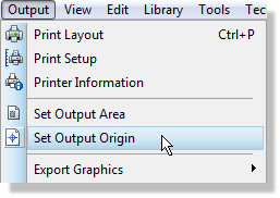
2) Move the mouse towards the bottom left of the board edge. Roll the middle mouse button as required to zoom in for more accurate placement.
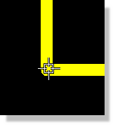
3) Left click the mouse to commit placement.
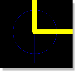
The co-ordinate display will now provide values relative to the position at the bottom left of the board by default, and relative to any specified temporary origin when set.
Remember that you can also toggle metric or imperial units via the command on the View menu or the ‘M’ keyboard shortcut.
A useful trick once we have specified our origin is to use the Goto Position command on the View Menu (CTRL+G) to move the mouse to the exact location we want to place position sensitive parts. This command will automatically switch between X-Y or Radius-Theta depending on whether you are in polar or cartesian co-ordinates.
The Proteus layout module has a default grid and will snap objects onto the grid, making it easy to form connections and control board layout. There are four hotkeyed snap settings for both metric and imperial units, changeable from the View Menu or by keyboard shortcuts. It follows that changing the snap setting to a lower unit will allow finer granularity, whereas raising the snap setting will make it easier to select objects at higher zoom levels. It is not advisable to change the snap settings regularly through a design but rather to choose the highest appropriate setting for the board you are working on.
You can change the four default snap settings via the Set Grid Snaps command on the Technology Menu.
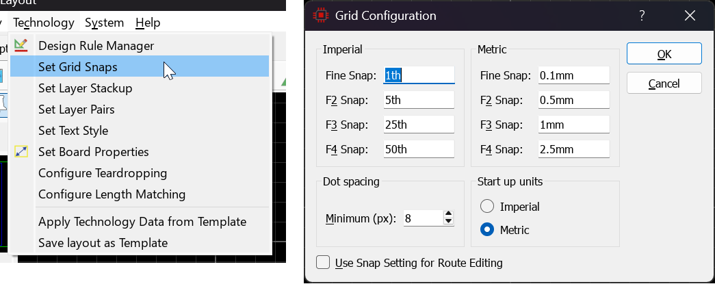
Grid settings can be set according to the users requirement
The grid display itself can be toggled between off, dots and lines via the ‘G’ key on your keyboard, whilst the colour of the grid can be configured from the Displayed Layers Dialogue (View Menu).
Measuring Distances
The origin and snap tools we have just seen let us place an object at a known co-ordinate. Very often though what we actually need is the distance between two things that are already on the board, for example the gap between a connector body and the board edge, or the spacing between two mounting holes. Measure Mode is the tool for this and it can also reposition one of the two objects to a distance we type in.
Measure Mode is the last icon on the mode toolbar, below the 2D graphics group. There is no default keyboard shortcut for it. When we enter the mode the Object Selector is replaced by the Measure Panel and all the other editing modes are suspended until we select a different mode.
Our board is empty at the moment so this is a safe place to try it out. Let us confirm the width of the board edge we drew earlier:
1) Select Measure Mode from the bottom of the mode toolbar.
2) Left click on the left hand side of the board edge graphic. The cursor snaps to the edge and a green arrow begins from that point.
3) Move the mouse across to the right hand side of the board edge and left click again. The arrow locks in place.
4) Read the values in the Measure Panel. The horizontal distance should be the 115mm we set when we placed the board edge.
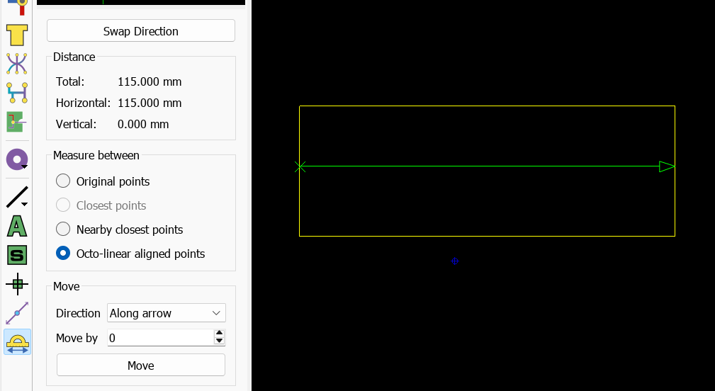
The Measure Panel reporting the width of the board edge, with the green measurement arrow running between the two clicked points
Both of those clicks landed on the same object, the board outline, so what we have measured is a dimension within one object rather than a clearance between two. The panel adapts to this: the Measure Between group offers only Original Points and Octo-linear Aligned Points, because the closest point between an object and itself is zero, and the Move group offers Move By, which offsets the whole object, rather than New Distance.
When the arrow does connect two different objects, all four Measure Between modes become available. Original Points measures between the exact points we clicked, which is what we want for centre to centre spacing. Closest Points reports the smallest gap anywhere between the two shapes. Nearby Closest Points reports the smallest gap in the region we clicked and is the best general purpose choice for edge to edge clearances. Octo-linear Aligned Points constrains the measurement to the nearest of the eight compass directions, which suits the horizontal, vertical and 45 degree geometry of a typical layout.
The snap considers only the layers that are currently visible. If the cursor keeps finding objects on a layer you are not interested in, hide that layer before measuring.
Underneath the distances is the Move group. With a two object measurement in place we can pick a direction, type the distance we want into New Distance and click Move, and Proteus repositions the object for us. We will use this twice as we continue: first to set the clearance between connector J2 and the board edge, then to place a mounting hole at an exact spacing.
Move always acts on the object at the tip of the arrow, so check which way the arrow is pointing before you click Move. It is easy to measure from a small object out to a board edge or a power zone and then move that large object by mistake. The Swap Direction button reverses the arrow so that the smaller object becomes the one that moves. If you do move the wrong thing, CTRL+Z will undo it.
Move repositions a whole object; it cannot alter a dimension inside one. We cannot widen the board with Measure Mode, which is why we set the board size by editing the graphic earlier. Note also that if the arrow tip lands on a pad belonging to a component, the whole component moves rather than the pad.
See Also:
Measure and Move (Reference Manual)
Measure and Move Examples (Reference Manual)
Placing Components and the Ratsnest
Now that we’ve handled all the basics we can finally start to get our components on the board. The following screenshot shows a fully placed board and we can use this to get our approximate positioning. Since it is a fairly simple board we are going to place manually but it is worth noting that Proteus includes a fairly sophisticated auto-placement facility that includes component grouping (e.g. powersupply, usbengine, etc.) and floorplanning on the layout. This is discussed in the reference manual via the link below.
See Also:
Auto-placement and Floorplanning
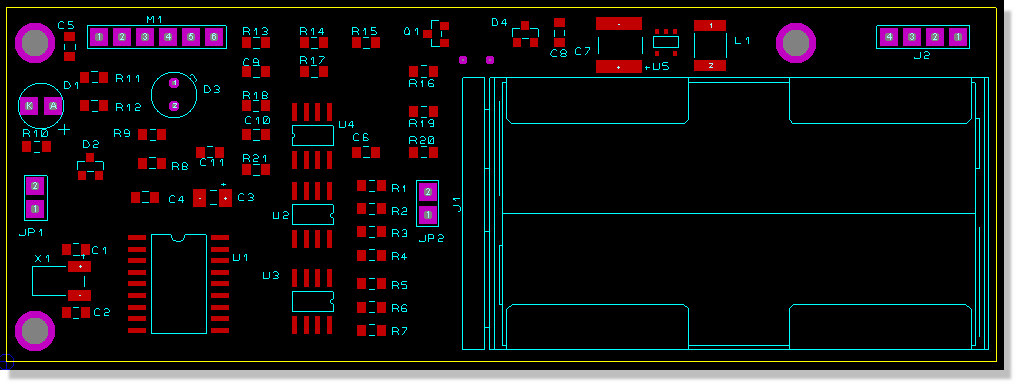
dsPIC33 board un-routed
Placing a component on the layout is very similar to that in the schematic module.
Start by selecting Component Mode from the left hand side icon set and then ensure that the layer selector is set to Component Side – we won’t be placing any solder side components in this project.
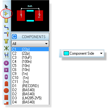
Component mode and the Layer Selector
The object selector by default will contain a list of all parts to be placed. For more complex boards however it is worth noting that you can restrict the display to only items selected on the schematic or only those on the currently selected schematic sheet.
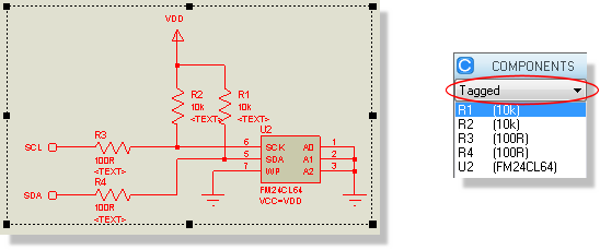
Components selected on the schematic can form a filtered placement list on the layout.
This allows you to select parts of your design in the schematic and then work on placement and routing of them on the layout without the clutter of other components in the object selector. Our layout however is relatively simple so we will work globally (all of the components available in the object selector).
Let’s get the AA battery holder down first on the right hand side of the board. Select J1 from the Object Selector, position the part using the previous screenshot as a guide and then left click again to commit placement. Note that once we have placed the part it is removed from the Object Selector and we can continue by placing the J2 connector above and towards the right of the battery.
You should notice both during placement and afterwards that there are green ‘elastic’ lines between the two components and also a yellow arrow from each component. The green lines are ratsnest lines and indicate connections that have to be made between the two parts, whilst the yellow arrows (named ‘force vectors’) indicate a preferred position for the part to minimise ratsnest distance. The force vectors are provided as guidance only and are based solely on logic to reduce ratsnest lines. Since we will be using the earlier screenshot to dictate positioning we can turn them off.
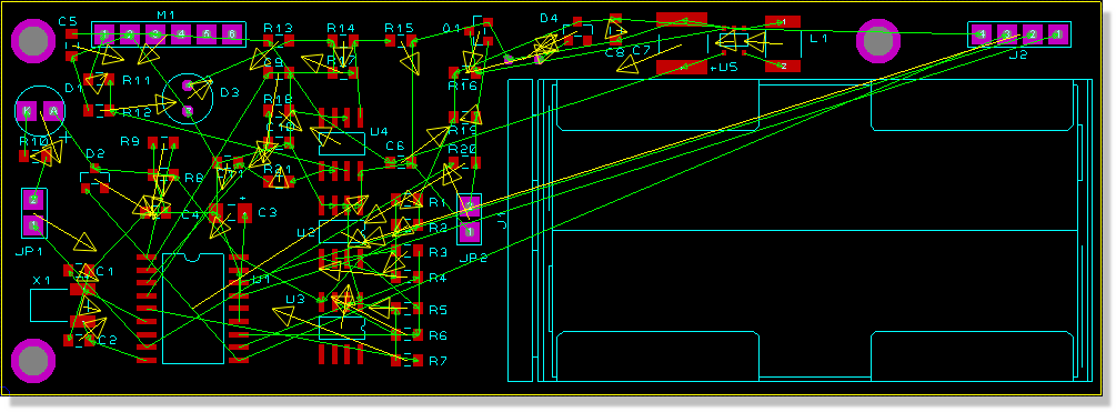
dsPIC33 board as you see it having placed all the components
From the View Menu, select the Edit Layer Colours/Visibility command. The resulting dialogue form shows all the available layers with colour and visibility configuration options. All we need do here is deselect the checkbox for the ‘Vectors and Ratsnest’ layer and exit the dialogue.
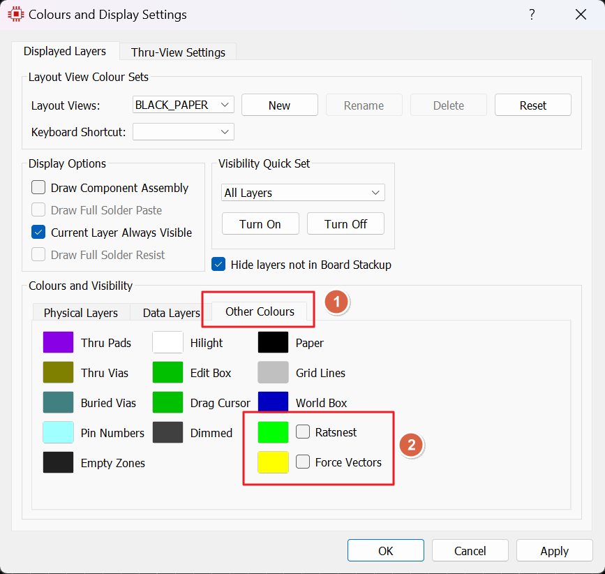
The Ratsnest and Force Vector layers turned off
You can also launch this dialogue form by clicking the mouse on the layers icon beside the layer selector at the bottom of the application window.
It is important to remember that this dialogue form controls visibility only; to control whether objects on a layer were selectable/editable we would use the Selection Filter which is discussed in more detail later in the documentation
See Also:
Ratsnest Features (Reference Manual)
You may find that you need more control over the positioning in order to move connector J2 into position. Remember that objects are linked to a snap grid so all we need do is reduce the snap grid via the options on the View Menu, for example to 1mm snap.
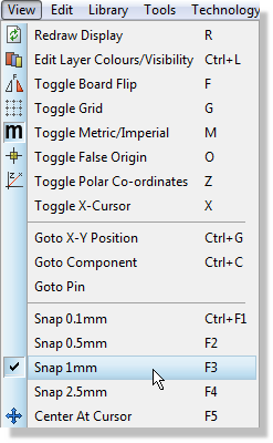
If you are working in imperial units you can either change the snap to 25th or use the ‘M’ shortcut to switch to metric units
Now that we have the granularity we need, simply right click on the part to select it and then drag it into the desired position. We can move the connector closer to the board edge if we move the part label underneath the part. Again, the process is identical to the one we covered in the schematic tutorial – remember this time to right click on the label itself and not the component body.
Dragging on a fine snap gets J2 roughly where we want it, but the clearance to the board edge is a mechanical requirement rather than a grid position, so this is a good place to use Measure Mode for the final adjustment. Say we want 1.5mm between the connector body and the board edge:
1) Select Measure Mode and left click on the courtyard of J2 (the boundary reserved around the component body), not on one of its pads.
2) Left click on the board edge segment beside the connector.
3) Select Nearby Closest Points. The panel now reports the edge to edge gap in the area we clicked, which is the clearance that actually matters for the case wall.
4) Click Swap Direction so that the arrow points at the connector rather than at the board edge. Without this step, Move would shift the whole board outline.
5) Set Direction to Along arrow, type 1.5mm into New Distance and click Move.
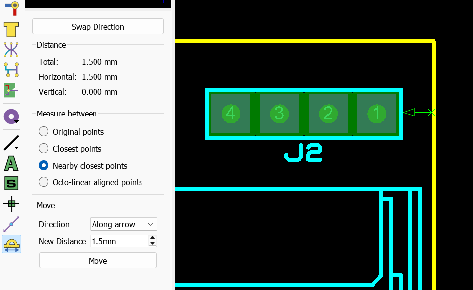
Measuring the gap between the J2 courtyard and the board edge in Nearby Closest Points mode, ready to move the connector to the required 1.5mm
The measurement updates as soon as the move completes, so we can see the result immediately. Switch back to Component Mode when you are finished, since Measure Mode suspends the placement modes while it is active.
As you place components and ratsnest lines appear the connectivity status also will update to show the number of missing connections.
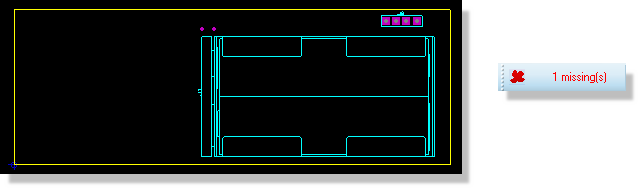
J1 and J2 placed with the CRC showing 1 connection missing
A missing connection is essentially a wire connection on the schematic that has not been routed on the layout. It follows that when the board is completed the connectivity status should report no missings. We'll look at this is more detail when we discuss routing later in the tutorial.
If we now consider the other principle components we can go ahead and place U1 (dsPIC33), U2 (I2C memory), U3 (temp/humidity sensor) and U4 (dual op-amp) in exactly the same way, such that we end up with something like the following screenshot.
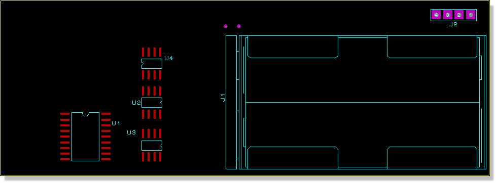
dsPIC33 board so far...
Note that the S08 footprints used for the U2, U3 and U4 components have been rotated appropriately to reduce ratsnest length. This is best done at placement time as the ratsnest display will update live to give visual guidance.
Start by placing U1 in the normal way and then start placement of U2 by left clicking once on the Editing Window. Now use the ‘+’ and ‘-‘ keys on your numeric keypad to rotate the component as you move it into position, left clicking the mouse again to commit placement as before. Repeat the process for U3 and U4, moving or rotating parts after placement (right click and then context menu options) until your board approximates the previous screenshot.
If you are placing components in a high density area where routing space is at a premium you can hide the part reference via the edit component dialogue form (right click on the part and select edit properties from the resulting dialogue form).
Generally speaking you have two options for placement of the board. You can either manually place the components in their positions or you can use the Autoplacement feature along with placement rooms to get all the components on the board in grouped locations. In either case, you may find it useful to temporarily disable the ratsnest lines during placement; remember that this is controlled from the Layers dialogue form as discussed earlier.
The auto-placer can be invoked from the Tools Menu in and for our purposes all the default options will suffice.
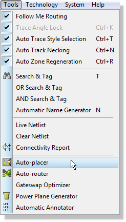
Selecting the Auto-Placer from the Tools menu
For more control over the placement of particular components we could draw out one or more placement rooms and then assign components to a particular room. This then better informs the autoplacer where to place given footprints on the PCB.
See Also:
Auto-Placement (Reference Manual)
Whichever route you follow the task is to lay out all the components on the layout, using the previous layout as a reference. Try to leave some space at the bottom of the board so that we can run traces down and along from connector J2
The following points are useful to bear in mind as you continue placement:
- The middle mouse will zoom you in and out as you place components (as will keyboard shortcuts F6 and F7)
- Right clicking on a component once placed will present a context menu option, allowing you to move, rotate or delete the part.
- Changing the snap settings to a finer grid will allow more accurate positioning at the expense of more precision being required to select the part.
- If you place a part in an illegal position (e.g. over another part) you will get one or more design rule violations. For now, simply move the part to a legal position – we will look more closely at design rules in the next chapter.

DRC errors
Once you feel comfortable with placing and moving parts, feel free to move on to the next section. We will load a board with all the parts placed before we discuss design rules and routing.
Mounting Holes and Pad Styles
Before we move on to look at connectivity considerations we should complete the physical layout by placing mounting holes for the board. In our case we want to use pad with a 3mm hole and a diameter of around 0.18in and to position them conveniently for mini-locking PCB supports. The first thing we need to do is switch into circular through hole pad mode and scan for a suitable pre-supplied pad in the Object Selector.
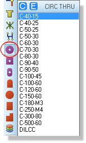
Select the correct pad style for mounting holes
The nomenclature of pads is designed for easy reading and tends to follow the following format:
<PAD TYPE> - <DIAMETER/SIZE> - <HOLE>
Units are in imperial unless prefixed with an ‘M’ so for example a C-40-15 is a circular pad with a 40th diameter and a 15th hole and a C-200-M3 is a circular pad with a 0.2in diameter and a 3mm hole. Our spec requires a pad with a 0.18in diameter and a 3mm hole, which we can see does not exist in the pre-supplied set. We therefore need to create the pad as follows:
1) From the Library Menu select the New Pad Style command.
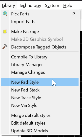
2) Enter a name for the pad; we recommend you follow the standard naming convention (i.e. C-180-M3).
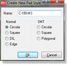
3) Specify the pad type – in our case we want Circular through hole pad.
4) The diameter of the pad is 180th or 0.18in. The drill mark is the size of the mark output in a drill plot, 30th would be fine. The drill hole needs to be 3mm and the guard gap should be enlarged to 20th. The guard gap (or solder mask expansion) is the amount by which the pad diameter is expanded on the resist plot.
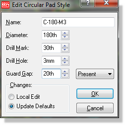
5) At the bottom of the dialogue form we have the choice whether to make this pad style permanent for future designs (Update Defaults option) or local only to this design (Local Edit option). Unless there is a particular reason for a local edit only we recommend that you leave this on the default setting.
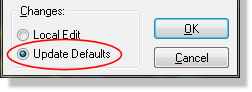
6) When you exit the dialogue form you should see that the new pad style is available for placement from the Object Selector.
When entering specific values you may find it easier to simply type in the values that you want rather than using the up and down arrows beside the controls.
Some parts need a hole that is not centred in its copper pad, USB receptacles and RJ-45 jacks being the usual examples. For drilled and slotted padstacks the Edit Padstack dialogue provides an Offset group with X and Y fields that displace the hole from the pad origin while the copper, resist and paste mask stay centred on it. See Off-Centre Holes in the reference manual.
We are going to want to place two mounting holes at the top and bottom left of the board and then a third at a specific location (for mini-locking PCB supports). You may therefore have to move some circuitry out of the way to make room; for example, the crystal block at the bottom or the pressure transducer at the top. As we’ve seen earlier we can easily do this by entering selection mode, drawing a selection box around the circuitry and then dragging to a new position. This is shown below with the crystal circuitry.
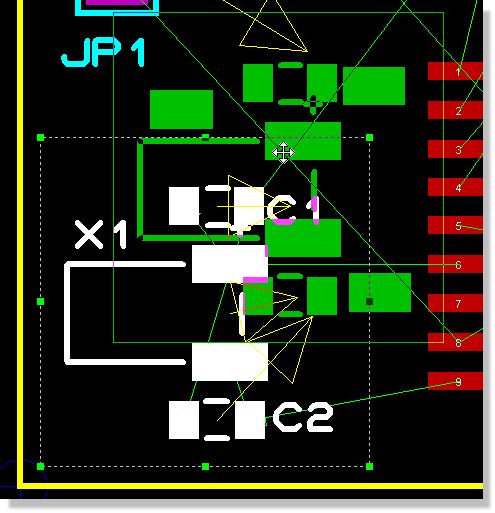
Moving a selection of circuitry
Remember that you can resize the selection box to include or exclude items using the drag handles if you don’t get the right size the first time.
Grouping Objects
A selection box like the one we have just used lasts only until the next click, and we will be drawing them repeatedly as the board comes together. The crystal and its two load capacitors belong together though, and we are likely to nudge them around more than once before we are finished. Rather than re-select them every time, we can make the association permanent with an object group.
With the crystal circuitry still tagged, right click inside the tagbox and select Group Objects from the context menu. The status bar confirms the new group and lists its members. The same command is available on the Edit menu.
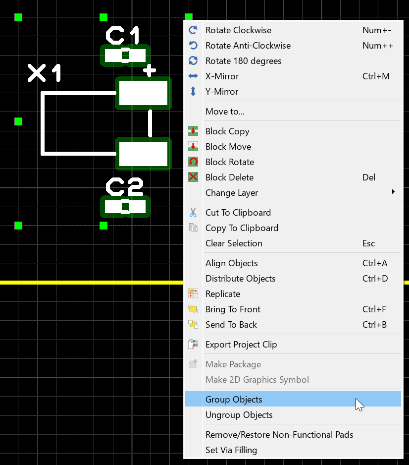
Group Objects on the context menu, with the crystal circuitry tagged ready to be grouped
Now drag any single member of the group. The whole block moves as one unit, and it will keep doing so for the rest of the design without us re-selecting anything. Rotate, mirror, Move To and the block commands all behave the same way. Repeat the exercise on the DC/DC converter circuitry if you need to move that out of the way as well.
Components, packages, 2D graphics, dimensions, zones, pads and rooms can all be grouped. Tracks and vias belong to the route database and cannot be group members, although tracks attached to grouped objects are rubber banded as normal when the group moves. Ungroup Objects, on the same context menu, dissolves a group again. The classic use for this is a connector together with its mounting holes and keepout graphics, which is very close to what we are doing here.
Deleting any member of a group via the context menu deletes the entire group. That is easy to trip over later on, so if you want to remove a single object from a grouped block, use Ungroup Objects first. We will meet exactly this situation when we come to cut the slot around U3.
Edit Properties always acts on the one object you clicked, so you can still edit a single component of a group without disturbing the rest. Distribute, Replicate and Change Layer likewise act only on the objects you select and do not expand to the whole group.
See Also:
Creating Object Groups (Reference Manual)
Once you’ve cleared some space, go to the circular PTH pad icon again, select the C120-100 pad style and place a single pad towards the top left of the board. Rather than place the second one by hand we can step a copy down the board with Replicate. Right click to cancel placement, then left click on the pad to highlight it and select the Replicate command from the Edit menu. Alternatively you can right click on the pad and select Replicate from the resulting context menu.
We want one copy directly below the first, so set the number of copies to 1, leave the X-Step at zero and enter a negative Y-Step that brings the copy down near the bottom left corner, in the region of -30mm on our board. Adjust the value to suit where you put the first pad; neither of these two holes has to be in an exact position.
Note that you need to include the units of either millimetres (mm) or Thou (th) when entering values in to the X/Y-step fields.
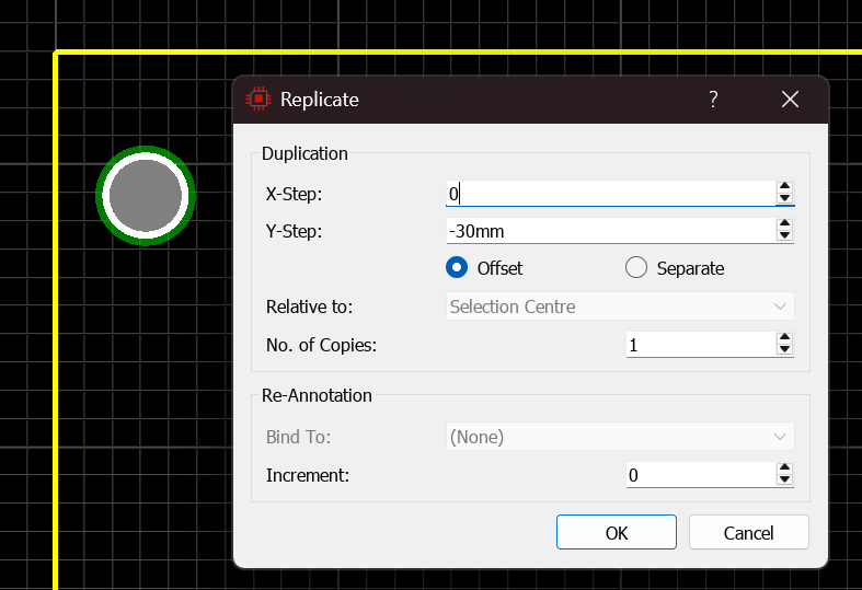
The Replicate dialogue set to one copy with a negative Y-Step, ready to place the second mounting hole
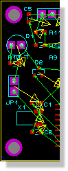
Mounting holes placed
The Replicate command on the Edit menu has options for automating tasks like stepping out a row of connector or LED pads at a fixed pitch, spacing copies by the gap between their edges rather than by the distance between their centres, and incrementing the reference designators as it copies. The spacing mode is set with the Offset and Separate options, and in Separate mode the Relative To control determines which bounds that gap is measured from, the component courtyard among them.
The third mounting hole goes above the battery and this one has to be accurate, because it carries a mini-locking PCB support that has to line up with the enclosure. The specification is 35mm up from the bottom of the board and 87.5mm along from the left. If required, move the DC/DC converter circuitry out of the way first, then switch back to pad mode and place the pad roughly where it needs to go. We will now measure it into position rather than trying to hit the co-ordinate readout with the mouse.
1) Select Measure Mode and left click on the bottom left corner of the board edge. The cursor snaps to the corner.
2) Left click on the mounting hole pad. The cursor snaps to the pad centre and the arrow tip is now on the pad, which is the object we want to move.
3) Select Original Points, since the specification is given from the board corner to the hole centre rather than as an edge to edge clearance.
4) Set Direction to Horizontally, type 87.5mm into New Distance and click Move. The pad slides along the X axis and keeps its vertical position.
5) Set Direction to Vertically, type 35mm into New Distance and click Move. The pad is now at the specified position.
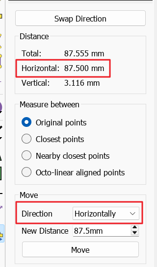
The Measure Panel showing the distance from the mounting hole to the board corner, with the move controls below
The horizontal and vertical readouts confirm the result straight away, so there is no need to zoom in and read co-ordinates off the status bar. Switch out of Measure Mode when you are done.
There are two other ways to do the same job. You can set a temporary origin at the board corner with the ‘O’ key and then chase the co-ordinate display up and right (you may need to switch into metric units using the ‘M’ shortcut key toggle). Or, having set the output origin and knowing the co-ordinates, you can right click on the mounting hole and select the Move To command from the context menu to position the part programmatically.
Grouping makes a set of objects move together. The complementary tool is Lock Position, which stops an object moving at all. With position sensitive components such as this mounting hole it is often useful to ensure that they cannot be nudged or moved inadvertently after placement. You can lock any object in position by moving the mouse over the object until it is encircled by a dashed line, right clicking on the object and selecting Edit Properties from the resulting context menu. The Lock Position checkbox can then be selected to prevent movement or deletion of the part.
You can also set a specific minimum zone clearance for the pad to reserve some extra space for the bolt.
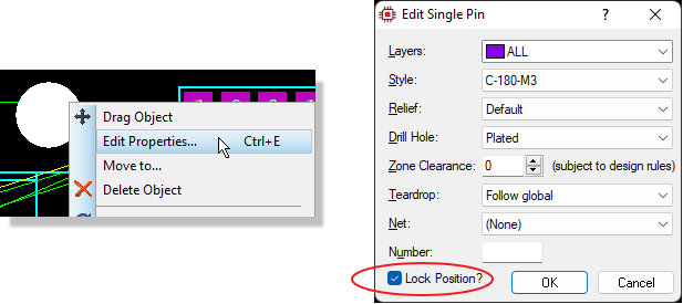
Locking pads and components
We have now completed the physical layout of the board. If you decided not to follow the full layout process you can load a version of the board in its current form by opening the home page, clicking on the Open Sample button. The project you want this time is the unrouted dsPIC33 Recorder project from the Tutorials category. Note that the pre-supplied project does not contain the object group we made earlier, so if you intend to follow the rest of the tutorial you should tag the crystal circuitry and group it (right click inside the tagbox, Group Objects) before continuing.
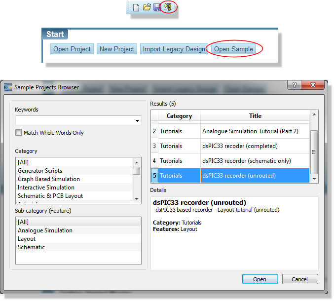
Opening a sample project
Design Rules and Net Classes
Now that we have a placed board we need to configure the software to obey any design constraints or electrical considerations relevant to the layout. We can do this largely from a single dialogue form called the Design Rule Manager. Start by launching this dialogue form now from the Technology Menu in the Proteus Layout module.
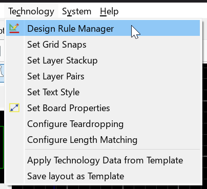
Design Rules
The first tab of this dialogue form allows us to configure constraints and minimum clearances for the layout. We have a DEFAULT rule loaded which must apply to all layers and all net classes, providing a set of clearances between objects equivalent to manufacturing guidelines.
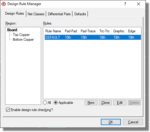
The Design Rule Manager
This rule and these clearances are created automatically for each layout in order to provide a minimum set of constraints for a board. You can change the values of the default clearances applied to new layouts via the Design Rule Manager on the Technology menu..
The first thing we need to decide is whether a single rule is suitable for all layers and all traces on the layout. It is possible to create as many new rules as required and we can limit their effect to a given layer on the PCB, a specific area of the PCB and/or a given set of connections (net class). A great deal of information on this is available in the reference manual but for our purposes we can manage fine with configuration of the existing rule.
Given that this equipment is intended to work out-doors we’ll need to increase the clearances between pads and traces to improve the insulation against condensing moisture. A 20% increase should be sufficient so we need to change the Pad-Pad, Pad-Trace and Trace-Trace clearances from 10th to 12th.
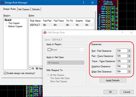
Default clearance settings in the DRC manager
The graphics and edge clearances are fine at the default values.
Note that the edge/slot clearance field defines the clearance for power planes against the board edge.
In addition to these clearances there are two board global rules, one Solder Resist Guard (Resist->Copper) and the other minimum solder dam (Resist->Resist). The Solder Resist Guard rule enforces a clearance between the solder mask and copper and is intended to prevent exposed slivers of copper on the manufactured PCB. The Min Solder Dam rule enforces a sliver of soldermask between pads and can help to avoid solder bridges. Since it's usefulness is dependant on board manufacturing techniques we've defaulted this rule to OFF.
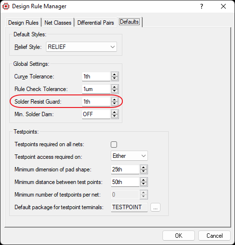
If, during route placement, you find these DRC errors, the solution is to either move the trace or edit the pad style and change the guard gap (solder mask expansion) for that pad style.
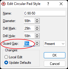
Editing the guard gap on a pad style to clear a solder resist violation
Two more global rules sit alongside these on the Default tab: Silk-Silk, which checks the clearance between silkscreen objects on the same layer, and Silk-Mask, which warns when silkscreen encroaches on a resist or paste mask opening. Both are off by default. Turning them on with legacy library parts can produce hundreds of violations, since older footprints often draw silk right up to the pads, so leave them off for now and enable them at final validation when you have time to deal with the results. The rules are documented under Silkscreen and DRC in the reference manual.
See Also:
Setting Design Rules (Reference Manual)
Design Rule Examples (Reference Manual)
Since there are no new rules required for this board we can move on to the net classes tab of the dialogue.
Net Classes
This is the place where we configure trace and via styles and control which layers we route on when auto-routing the board. The selector at the top allows us to switch between different net classes and configure each separately.
Let’s start with the POWER Net class, which should be the default selection. As we discussed in the Schematic Getting Started Guide any nets that include a power or ground terminal are automatically assigned to the POWER net class, unless manually overridden.
We’ll set the track / trace size to 25th, not so much for current considerations but to reduce track impedance (we’ll also place a single low impedance ground plane later to help with this). In Proteus nomenclature this corresponds to track style T25.
The neck style – if configured – specifies the track style for necking (thinning) to help the track pass through obstacles. Together with our design rule aware routing (which knows which objects are obstacles) this is very powerful. When set, you can use SHIFT+N to toggle between necked and normal track styles during routing which is invaluable in tricky or dense board areas.
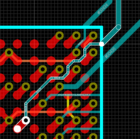
Advanced necking: SHIFT+N is toggled on while routing the escape from the BGA and then toggled off again to resume routing at normal track width.
The status bar will update to show that you are using the neck style as well as show you it's thickness.
Our board is not likely to be complex enough that this will be an issue but we'll set the neck style to 15th so that we can practise.
Given that we don’t really have current constraints the choice of vias is a trade off between the higher manufacturing costs of smaller vias and the decreased routing quality of large vias. For the current this circuit is dealing with and for a standard 1.6mm FR-4 support plated with 35um copper, vias with the standard 0.4mm hole are a good compromise. For the power tracks we need a suitable annular size and 40th is a reasonable choice. We can therefore set the via style to be V40.
If you are not sure of the characteristics of a particular style, you can view them by selecting the appropriate mode icon (via, track, pad, etc.), highlighting the style in question in the Object Selector, and then clicking on the ‘E’ button at the top of the Object Selector.
The options at the bottom of the dialogue form allow us to change the via type and also to change the colour or visibility of the ratsnest lines. The ratsnest settings can be useful if we are manually routing and wish to quickly distinguish between power and signal connections. There is nothing to choose in the via type on a two layer board, where every via is a through-hole via, but on a multi-layer or HDI board this is where you would select blind, buried or micro-via styles for the class.
The layer assignment pairs on the right hand side tell the autorouter which layers to route on for multi-layer boards. Again, for our two layer board, there is nothing to configure here.
We should now have finished setting up the POWER net class – your dialogue form should now be configured as per the following screenshot.
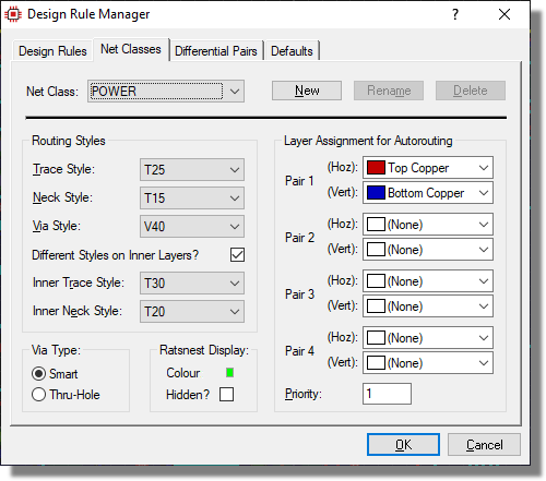
Specifying the Power net settings
Lets move on to the next net class in the selector; the ANSW class. You may remember that we specifically named this net class in the Schematic Getting Started Guide in order that the 5V switched power supply for the analog circuitry (the output of the DC/DC converter) could be handled separately. What we want for these connections is a track size larger than the standard SIGNAL net class but smaller than the POWER net class, so lets change the Trace Style to T15 (15th track). For consistency, the neck style can also be T15 and we can use a smaller via (with the same 0.4mm hole) by selecting the V30 Via Style.
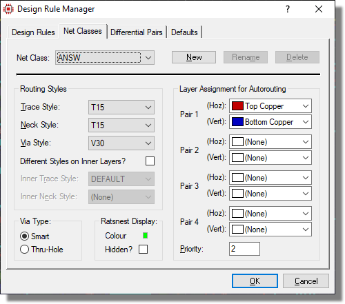
Specifying the ANSW net settings
If you don’t have a V30 via style you can create one easily by going to the Library Menu, selecting New Via Style and filling out appropriately.
Creating your own net classes on the schematic is extremely simple and provides you with the flexibility you need both with regard to trace and via configuration but also with design rule constraints
The final net class we have is the standard SIGNAL net class that encompasses all non-power and unspecified connections. We’ve deviated from the widely used “8/10 Rules” (8th trace, 10th clearance) in order to compensate for outdoor usage but the standard 8th track width (style T8) is fine. We can also set the neck style to 8th and keep our standard V30 via style for these connections.
Having finished configuration, exit the dialogue form to return to the layout.
See Also:
Net Classes (Reference Manual)
Keepout Areas
We can also introduce tracking constraints by limiting areas in which tracks can be placed. A good example of this is the crystal towards the bottom left of the layout where we do not want tracks under this area. To form a keepout area, start by selecting the 2D Box graphic icon and changing the layer selector to be keepout.

Selecting the Keepout layer
Next, place a small box around the silkscreen of the crystal in exactly the same way as we did for the board edge (left click to start placement, drag out the area, left click again to commit placement).
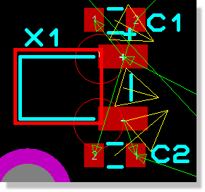
Keepout placed produces 2 DRC errors
Unless you are very skillful you will be presented with a box indicating that design rules have been detected.
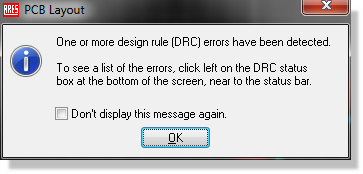
First DRC warning
Checking the box on the dialogue form will prevent it from appearing in the future. If you left click the mouse on the DRC section of the status bar a small window will appear providing information on the errors. You should see that they are of type PAD-EDGE as the pads of the crystal are closer to the keepout graphic than the 15th specified in the Design Rules.
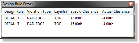
Displaying DRC errors
We have two options here:
1) Ignore the DRC errors. The keepout graphic will not impact on connectivity. If you want to do this, right click on the error and select Ignore from the resulting context menu.
2) Move the graphic to a legal distance from the pads. The easiest way to do this is to first change the snap level down (View Menu), right click on the graphic and select the Drag Object context menu option, and then change the snap level back when you are finished.
When you are finished your keepout area should look something like the following screenshot.
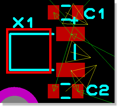
Correctly placed Keepout
The default for the keepout is that it applies to all layers. However, after placing the graphic on the keepout layer, you can right click change it to apply only to a specific copper layer from the resulting context menu. This can be very useful on more complex or densely packed board.
This keepout belongs to the crystal, so it ought to travel with the crystal if we ever move that block again. Draw a tagbox around the crystal circuitry and its new keepout graphic and then right click and select Group Objects. Tagging any member of the existing crystal group expands the selection to the whole group, so the result is one block containing the parts and the keepout graphic together. Drag any of the parts to confirm that the keepout now comes along with them.
We have a similar problem around the temperature/humidity sensor (U3). We are going to want a slot machined on the board to cut the thermal path and reduce the measurement errors of the sensor (we want to measure environment temperature, not the one conducted by the PCB). We therefore need to ensure that no tracks are placed in the area we are going to slot through:
1) Select the 2D Graphics rectangle icon and then change the layer to be KEEPOUT.
The 2D box mode icon with the layer selector set to the keepout layer
2) Place a rectangle around the bottom half of the IC as shown below.
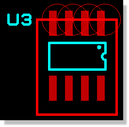
U3 with a Keepout
This time we cannot move the keepout to remove the DRC errors as the positioning is sensitive. Instead we can manually override the errors by launching the DRC dialogue, right clicking and selecting the Ignore option from the resulting context menu.
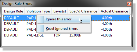
Ignoring DRC errors
Alternatively, we can designate this area of the board to have different design rules from everywhere else. To do this, we select the room icon and drag a box around the area. Then we set it up as a DRC room which needs to cover all layers (since the keepout is on all layers) and give it a sensible name.
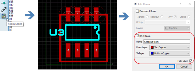
Setting up a Design Rule Room
Now that we have the room set up we need to change the design rules inside it. Go back to the design rule manager and find the room definition. You'll notice when you select the room in the tree that the right hand side shows you the default rule but shaded in a light grey. This indicates that the default rule applies in the area but was defined at a higher level. In other words, the room inherits the clearances from the board unless you give it specific clearances. We do this by clicking on the new button to create a new rule, give the rule a name and scope it to apply to the room and finally setting the clearances we want. In our case we simply want to turn off the edge clearance test in this area - everything else can stay the same.
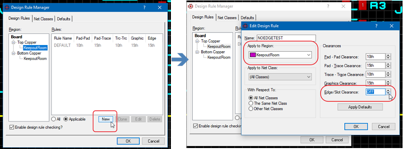
Setting a new Rule for the Design Room.
Design Rooms are a really useful concept and helpful wherever clearances vary in specific regions of the PCB. This can be as simple as pad-pad clearance on fine pitch SMD devices, fanout areas from BGAs, edge connectors at the board edge and so on. We strongly recommend you read up further in the reference manual.
A room that belongs to a particular part should move with that part, so this is another place for Group Objects. Tag the room and U3 together and group them, and the rule area will follow the sensor wherever it goes.
Grouping a room with a component is also the mechanism behind an exclude foreign room. With Exclude Foreign enabled the room voids any zone fill inside its boundary and flags any copper that does not belong to the grouped component as a DRC violation, which replaces the old trick of drawing an empty zone on each layer to hold copper off. Typical uses are the void beneath a magnetic part and a connector with a specific clearance envelope.
On an HDI board a DRC room is also how micro-via styles are applied to a region. The room carries a via style override, so vias dropped inside it during manual routing take the room's micro-via style wherever the layer transition allows. Since the autorouter only ever uses CNC drill spans, the Apply Style button on the room converts the vias it placed afterwards.
See Also:
Routing the Board
Having configured the board constraints we can now move on to actually making connections and routing the board.
Most of the pre-routing checklist that the reference manual sets out is now behind us: we have placed a board edge, defined the layer stackup and drill spans, set the design rules and, on an HDI board, set up any micro-via rooms. The two remaining items, layer pairs and power planes, are covered shortly. If you find yourself starting a board of your own and wondering what to do first, that list is the order to work in.
See Also:
Pre-Routing Checklist (Reference Manual)
Teardrops & Tapering
Placing teardrops at the connection point between track and pad is often useful in preventing drill breakout during board manufacture. We can configure teardrops from the Configure Teardropping command on the Technology Menu.
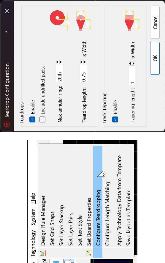
The dialogue form lets us set the maximum annular ring size on a pad below which a teardrop connection will be made and then also lets us set the length of the teardrop. You can, if you want, also apply teardrops to surface mount pads although we are not aware of any manufacturing reason for doing so. On surface mount pads the annular ring parameter is considered to be center pad to nearest pad edge.
You can also taper the tracks. This option sets the preferred length for the track taper based on a percentage of the width of the thickest track (to ensure consistency across the board).
A per pad override for setting/clearing a teardrop connection can be accessed from the edit single pin dialogue. This provides an additional level of control over where teardrop connections are made.
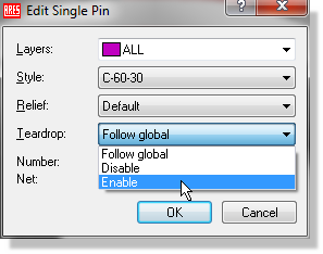
Note that the creation of a teardrop connection is dependant on the design rules. If making a teardrop connection would violate one of the design rules then it will simply not be created.
Once configured teardrops connections will be made dynamically as we complete routes in the sections below.
Tutorial Movie : Using Teardrop Connections in Proteus.
Placing a Route Manually
Before we start, we will want the ratsnest lines turned back on. If you have them disabled (can't see any green lines between pads), turn them on from the View Menu - Displayed Layers dialogue.
Let’s begin by manually placing some tracks on the board. Typically, we would manually lay out connections where a specific path is desired for the track or where we need greater control over track position. On our layout we want to make sure that our connections from connector J2 follow a sensible path around the board so we can start here and route them manually.
Start by selecting track mode at the left hand side of the Object Selector and changing the layer selector to be on Top Copper.
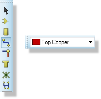
Trace / Track selection and the Layer selector
If we look at pad 4 of the J2 connector we can see that the closest ratsnest line is directing us across to the GND pad on the step converter. This is not ideal as we would have to navigate the mounting hole and then track into the small SMT pad. Instead, we will route this down and across the bottom of the board to a more convenient ground connection.
Proteus comes with two main routing modes, namely Push mode and Follow-Me-Routing Mode (FMR mode). Both will obey all of the design rules for the board that we set up previously. Push mode will allow you to nudge or move other tracks and vias out of the way to make space for the track being placed. It is almost always the fastest way to route a board and particularly so for densely packed boards. FMR mode is a sophisticated 'follow me' routing algorithm for manual routing in which the route being placed will follow the path of the mouse and hug obstacles at the clearance boundaries.
You can toggle between push mode and FMR mode using the SHIFT+P keyboard shortcut.
You start track placement by left clicking the mouse on pad 4 and then move the mouse downwards.
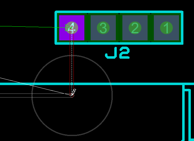
Routing J2 Pin 4
Notice that the routing mode and length are shown on the status bar.

You'll also notice an enlarged circle around the mouse pointer. This is called Visual DRC and will show you the design rule clearances of all obstacles inside the circle - really helpful in plotting your route path across the board.
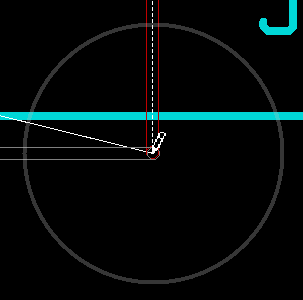
You should see that the closest legal destination for the track is now highlighted with a white line or a white arrow.
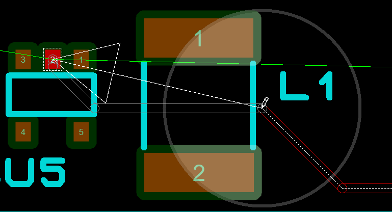
If there are no destinations on the current layer the indicator line will appear dashed but will still show you the nearest legal destination for the current route.
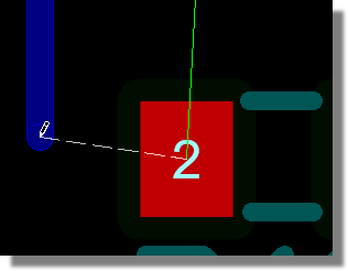
This will update as we move the mouse and since we are not going to route to this destination we can ignore it for now.
When a destination is available on the current layer you will see a shadow track between the current mouse position and the destination. If you press the ENTER key on the keyboard it will complete the route along the path shown by the shadow track. You can do this at any time while routing manually. This click to complete functionality can be turned off manually from the Route Command Centre on the Tools Menu or 'R'.
When the mouse approaches the bottom of the board, you could just change direction to the left and the track will corner to follow the mouse. However, since we want a tighter corner it is better to left click the mouse to place an anchor and then change direction to the left.
You will see that as we move further to the left the ratsnest guide will change to show us that we can terminate the track on pin 1 of jumper JP2.
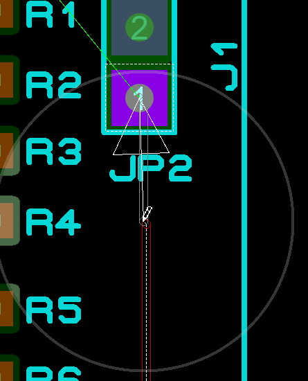
Connecting to JP2 Pin 1
Once we are underneath the jumper we can change direction and move upwards towards the destination pin
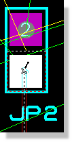
Connecting the trace to the pin
Finally, we can click left over the pin to finish placing the route. This will both commit the route and remove the ratsnest line corresponding to this connection.
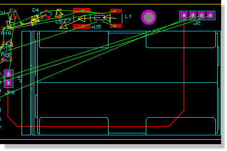
Finished route from J2 pin 4 to JP2 pin 1
Note that we did not need to select the width of track to route with as we configured this in the previous chapter. Proteus recognises that we are routing a track on the GND net, applied the rules for the POWER net class and selected the specified 25th track style for us.
Manual routing is probably the most common action you will perform with the software and it is vital that you understand how it works. The basic rules of operation are :
- Left click on pad, track or zone border to begin routing from that object.
- SHIFT+P key toggles between push mode and FMR mode. Status bar tells you which you are in.
- Left click at any point during routing to commit the route up to the mouse position (we call this anchoring).
- Right click to terminate the route at it's last committed / anchored point.
- ESCAPE key to abandon route entry completely.
- ENTER key will automatically complete the track in the path shown by the 'shadow' track.
- SPACEBAR to float a via on the end of the route and left click to then place the floating via.
- Double left click to drop a via at the current mouse position.
- Move the mouse backwards over existing tracking to rub-out.
- SHIFT+N key toggles the neck style on/off.
- SHIFT+C key toggles curved tracking mode on/off (only available in FMR mode).
- R key launches Route Command Centre to configure routing modes and styles.
Route Command Centre
Route command centre is a central dialogue form which offers full control of routing modes and styles. It can be launched using the R keyboard shortcut at any time - including in the middle of placing a route.
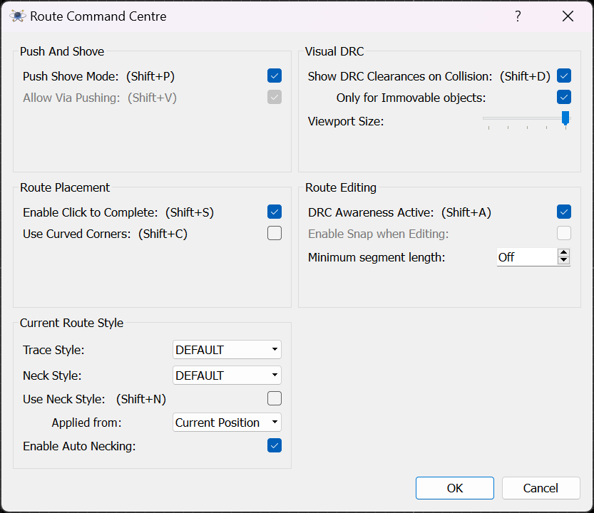
Push and Shove
These commands toggle push mode on and off (SHIFT+P) and apply to both route placement and route editing.
- When push mode is on the track being placed or edited will move other tracks (and vias where selected) out of the way while maintaining design rule clearances.
- When push mode is off, route placement happens in FMR mode where you can hug other objects but not move them. Route editing is similarly unable to move other objects on the board.
Normally, you would toggle this option directly from the shortcut key with the current mode being shown on the status bar.

The via pushing option then allows the route being placed or edited to not only move tracks but also vias as well. It's very useful but it can disturb routes on more than one layer and therefore require more tidy up. Generally speaking, it's best left on since most via pushes are small nudges.
Route Placement
These options are specific to route placement and apply regardless of whether Push mode is enabled or not.
Click To Complete is toggled via (SHIFT+S) and provides a calculated solution to the destination shown as a 'shadow track' in front of the route being placed. You can complete the route at any time by pressing the ENTER key.
Routing with curved corners can be toggled via (SHIFT+C) and switches the corner type from mitred to curved. You can also choose to change the cornering type of individual or all tracks from the mitre command either on the track context menu or globally on the tools menu. This will present an option to switch the cornering type between curved and linear.
Current Route Styling
The bottom left section of the Route Command Centre allows control of track width and neck width while in the middle of placing a route. These options will all be disabled unless you are in the middle of route placement, so to use them you would:
- Start placing a route.
- Press R to launch the Route Command Centre
- Change route and neck width as needed
- Exit the dialogue form and continue route placement.
- Repeat at a later point in the route as needed.
By far the most common use of these options will be to toggle necking mode on and off as you route a track in and out of a dense area. You don't need to go into Route Command Centre to do this. SHIFT+N shortcut key will toggle neck style on/off and the status bar will update to show both when you are in neck style mode and also the length of the current neck routing.
Route Styles come from the Net Class as set in the Design Rule Manager. The overrides here allow in route modification but are not intended to be a substitute for setting up net classes properly.
Route Editing
The route editing options are primarily concerned with design rule awareness. By default, track editing operations are design rule aware. This is almost - but not always - what you want to happen and will make tidying up the PCB a much easier job. However, sometimes you just want to get things out of the way and are prepared to deal with violations at a later point. If this is the case you can either turn off the DRC awareness off completely or tailor it to ignore components for example when editing tracks.
DRC awareness needs to be turned on in order to push other routes when editing. If DRC awareness is off there are no obstacles to push (Proteus is blind) and you can edit into an illegal position.
Visual DRC
Visual DRC provides a viewport around the mouse and each object shows an expansion corresponding to it's design rule clearance in an overlay. This instantly lets you see whether the route being placed/editing can move where you want it to go and then take action such as toggling push mode or changing track style to squeeze through a tight gap. These options allow you to adjust the size of the Visual DRC circle, turn it off completely or enable it for all objects instead of only immovable objects. The latter option is a little subtle because it depends what mode you are in. In push mode, most tracks and vias can be pushed and are therefore not immovable. This is normally helpful because you can see at a glance both where you cannot go (immovable with DRC clearance) and where you can force your way (pushable objects). In FMR mode, all objects are immovable and therefore always show their clearances.
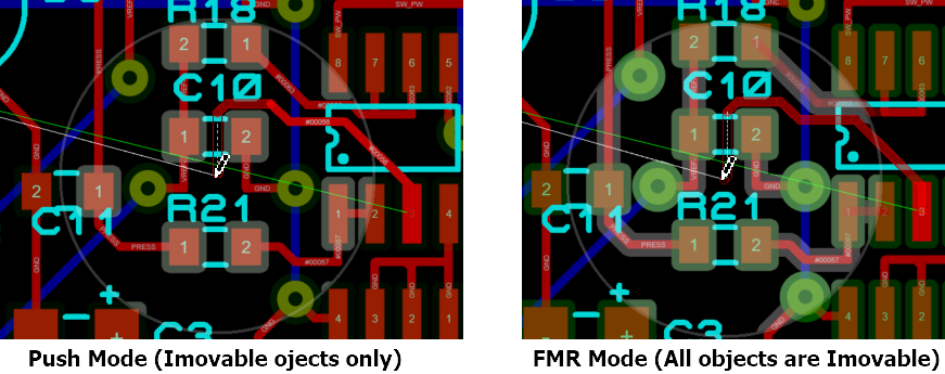
You'll find detailed help on all of the fields in the dialogue level help accessed by the question mark icon at the top right of the dialogue form.
See Also:
We strongly recommend experimenting with manual routing for a while on this board until you are comfortable with how it works in both main modes. You'll probably find that initially you use Route Command Centre to make changes to routing modes but over time you learn the main keyboard shortcuts and then use them directly. The following is a summary of how to perform common actions; try these while routing any of the remaining connections.
Switching Modes
Switch between push mode and FMR mode using SHIFT+P and verify on status bar which mode you are in. Push mode will be your primary tool but FMR mode may occasionally be useful as well.
Panning and Zooming
While placing a track you can use the middle mouse wheel (or F6 & F7 keys) to zoom in and out during routing. Panning will happen seamlessly when the mouse is at the edge of the Editing window during routing.
Placing Anchors
The routing algorithm will move the track being placed according to the way you move the mouse. If you want a track to follow a particular path then you need to help by left clicking whenever you change direction. This places an anchor or commits the route up to the mouse pointer such that the follow me router will not change it. You will see this happening as the outline track becomes solid.
Getting Stuck / Re-routing while routing
Since the manual routing system obeys the design rules for the board you don't need to worry about clearances while placing routes. You can however route to a place where you are blocked (the routing icon will change to a no-go sign at this point). Often you just place a via and continue on but sometimes it is better to rewind and try another path across the current layer.
Moving the mouse backwards over the route being placed will rub out that portion of track so to rewind and change direction just move the mouse back to the last good point - anything you had placed from that point onwards will be removed.
On densely packed boards in particular, speed of mouse movement is an issue. Remember that you are guiding the placement so moving slowly through tight spaces will work far better than ripping the mouse from source to destination. Use the SHIFT+N key to toggle in and out of neck style - this will get you through tight spaces.
Placing Vias
If you double click during placement you will place a via at the point the mouse is at and can then continue routing on the associated layer. If you press the spacebar you will float a via on the end of the mouse and can then position the via manually before placing with a left click. Using the spacebar has the advantage of snapping to legal objects (e.g. via under SMT).
In either case the placement of the via is also design rule aware and the PCB editor will not let you drop a via in an illegal spot. If you use the floating via method (with the spacebar) Proteus will attempt move the via to the nearest legal spot. This can be extremely useful on busy boards or when you want to butt a via tightly against another object.
Layers used for vias are defined by the Set Layer Pairs command on the Technology Menu. Examples of routing with vias and discussion on layer pairs follows further in the tutorial.
On HDI boards with a 1+n+1 stackup, Proteus supports micro-via styles for the laser-drilled outer layer transitions. Micro-via styles can be created from the Library menu and assigned through DRC room via style overrides in areas where micro-via routing is required. During manual routing, the system will automatically select the appropriate drill span based on the layer transition being made. The autorouter uses only CNC drill spans; after autorouting, use the Apply Style button on each DRC room to convert vias to micro-via styles. See the reference manual for full details on micro-via styles and via-in-pad filling.
See Also:
Object Hugging
It's often easier to use FMR mode (SHIFT+P to toggle) to hug a track to another track or to wrap a track around an object. If the mouse is over an object where the route being placed cannot travel then the route will follow the mouse path as closely as it legally can, essentially hugging the barrier object.
You can hug in push mode but only if the object you are hugging cannot be pushed !
Abandoning a Route
- If you want to abandon the route at the last committed (solid) segment then right click the mouse.
- If you want to abandon the route at the mouse pointer then left click to commit up to mouse pointer and then right click to terminate the track.
- If you want to abandon the route completely then hit the ESCAPE key..
Making Connections
If you are connecting directly to a pad then a left click of the mouse will complete the connection and terminate route placement.
If you are connecting to a track then left click will commit the placement and right click will terminate the route forming the connection. The same procedure applies if you are connecting to a zone except that you must connect to the zone border.
See Also:
Route Placement & Editing (Reference Manual)
Manual Routing Examples (Reference Manual)
Placing a Curved Route
Placing a route with curved corners can be helpful with signal integrity and net tuning or simply for aesthetic reasons. In Proteus, curved routing is only possible in FMR mode. So,
1) Left Click the mouse to start the route.
2) Check status bar and SHIFT+P to toggle into FMR mode if necessary.
3) SHIFT+C to toggle on curved corners and guide the route towards the destination pad with the mouse.
4) Left click the mouse on the destination pad to terminate the route.
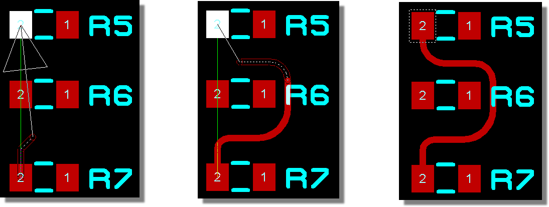
Deleting a Route
Once the route has been completed we can delete either the full route or a specific part of the route if we are not happy with the placement. Let’s assume that we were not happy with our placement of the last piece of track (upwards to pad 1 of JP2).
Start by right clicking on the track over this segment of track. This will highlight the entire track and the Delete Route option near the top would then remove the complete trace from the board. However, we have far more control if we use the options at the bottom of the context menu. In this particular case, select the Trim to Single Segment option; this will change the selected area of track to the segment we have clicked on.
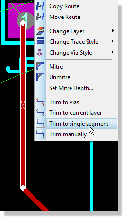
Trimming a trace to a single segment
Next, right click on the highlighted segment and select the Delete Route command; this will delete only this segment of the route.
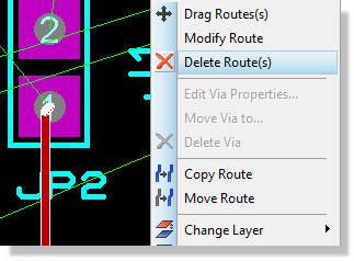
Deleting a trace via the context menu
Finally, zoom in, change the snap settings if need be and replace the route from the existing track to the terminating pad.
If things have gone more badly wrong you can simply delete the entire route and start again; what you are aiming for is something like the following screenshot:
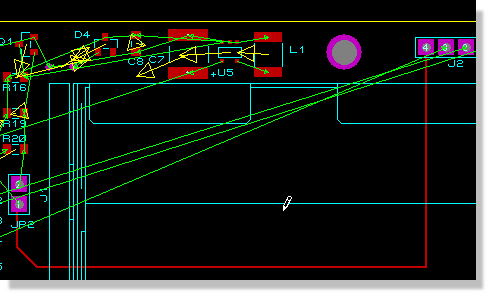
Editing a Route
It is often the case that routes need to be nudged or moved into position after placement and we definitely don’t want to be deleting and replacing routes or parts of routes all the time. To take an example, lets move our track lower down the board a little, towards the bottom board edge.
Start by right clicking on the horizontal section (segment) of the track; this is the section we want to move. Next, select Drag Route from the resulting context menu, move the mouse down to ‘pull’ the track into the desired location and then left click again to commit placement.
Moving tracks works as we’ve seen on a track segment. Using the Trim Manually option on the context menu for a track allows you to define your own segment and you therefore have complete flexibility with altering track topology.
Multi-Track Route Editing
For multi-track editing where the route being dragged hits another route the rules for route editing behaviour can be broadly summarised as:
- When Design Rule Aware Editing is on (the default) the system knows about other objects on the board and will avoid violations. If you turn this off Proteus is entirely blind and you can edit a track anywhere, including through other tracks and components.
- When Push mode is on (the default) editing tracks will push other tracks out of the way so long as Design Rule Aware Editing is on. When Push mode is toggled off editing tracks will hug other tracks so long as design rule aware editing is on.
The most common usage is likely to be in push mode as that will maximise space on the layout. However, there are times when you want specifically to hug another track and toggling push mode off will do that.
| Shortcut | Action |
| SHIFT+P | Toggles push mode on and off. Note that this setting applies to both route placement and route editing. |
| SHIFT+A | Toggles design rule aware editing on and off. This should only really be turned off if you are in a position where a legal edit is impossible (e.g. you've changed pad->track design rules and existing tracks are in violation) |
| R | Launches the Route Command Centre where all route options can be found |
Changing Widths
You can also make route edits that aren't related to dragging tracks. The obvious example of this is changing the width of the track(s) and/or the via style used when routing them. You can do this by first switching to selection mode, then using CTRL+left click to select and finally by right clicking on any of the selected tracks to access the context menu.
You can drag segments and curves when editing a curved route in the same way as you would drag segments and 45 lines in linear routes.
DRC Aware Editing vs Guided Route Editing
Route editing by default is fully design rule aware so you can only move tracks in legal places but you can toggle this via the SHIFT+A shortcut or in the Route Command Centre (R key shortcut). The DRC awareness will be shown along with the edited track length on the status bar. When DRC awareness is turned off then Visual DRC helps with route editing in two ways.
- The border of the Visual DRC viewport will highlight whenever any part of the route is in violation. This is an important indicator, particularly on large routes where the route segment in violation may not be the one you are editing or where editing brings the route into violation somewhere outside the screen area.
- Trace segments and objects which are in DRC violation with the currently edited route inside the viewport will be highlighted. This allows for fine control during editing, allowing you to zoom in and carefully position the route without creating a DRC error.
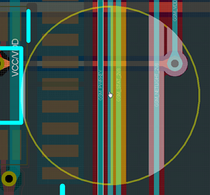
Violation inside the viewport area is highlighted.
See Also:
Reference Manual: Manual Routing Examples.
Reference Manual: High Speed Routing Examples.
Layer Pairs and Manual Routing
The track we have placed is of course only on top copper, whereas we often want to via up and down through the board when routing. Proteus handles this with a concept called Layer Pairs. This means that every layer on the board has an associated layer so that via destinations are known during placement. For a two layer board this is obvious with top copper being associated with bottom copper and vice versa but with multi-layer boards configuring the layer pairs (Technology Menu, Set Layer Pairs) can be an important step.
Don't be surprised to see much of the layer pairs dialogue disabled. The available layer pairs are restricted to the signal copper layers set up in your layer stack.
See Also:
In our case, the default assignments are correct and no action is required. Let’s place a couple more routes manually to see how this works. We’ll look at connecting pins 1 and 2 of the J2 connector which are the transmission lines from the USART on the dsPIC processor.
We’ll start with pin 1 and route from the pin on the bottom copper layer. Make sure that you have track mode selected and then hit the space bar on the keyboard, noticing that this will toggle the layer between the two layers associated as a layer pair. If you have ended up on top copper simply hit the space bar again to set the layer to bottom copper.
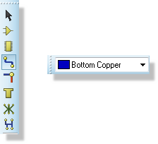
Selecting the Bottom Copper layer
The processor is some distance from the connector and the easiest path would seem to be down and along the bottom of the board. Begin placing the track by left clicking on pin 1 on the connector and then moving the mouse downwards
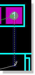
Routing on Bottom Copper
When we get near the bottom of the board, left click the mouse to place anchors and guide the mouse to the left. To maximise space on the board you can route across the bottom of the board with the mouse over the board edge graphic - this will hug the track to the absolute edge of the board leaving only the Edge Clearance between the two.
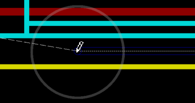
Tracks will hug the board edge
Once you get near the U1 IC bring the track up just past the right hand pads of the processor footprint.
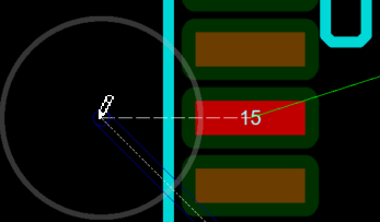
Routing to the left of the right hand pads of the Processor
We now need to place a via before we can connect to the SMT pad on top copper. As described above you can either double click the mouse at the point you wish to place the via or you can press the spacebar to float a via and then guide the placement point with the mouse before left clicking to commit. The latter method has the advantage of allowing you to butt the via as closely as possible against the pad thereby minimising the stub track length on top copper.
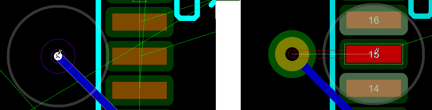
Placing a via by pressing the space bar
Quite a lot has been covered in making these connections and, unless you are fairly skillful, there has probably been some finger trouble along the way. We’ll continue with the other connections from the J2 connector to help familiarise ourselves with the techniques we’ve introduced.
Pin 2 of the connector should follow an almost identical path to pin 1 and again we can start placement on bottom copper (check the layer selector before you start placement; the space bar will toggle the layers). We can either push the track towards the board edge and then hug (if in push mode) or simply hug the track we have just placed (if in FMR mode) by moving the mouse parallel to the path we want to travel but over the original track as shown below.
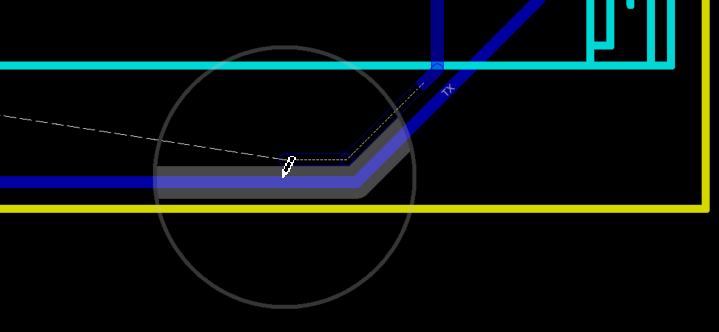
Tracks will also hug other tracks
In order to make the connection, we can then route vertically underneath the pads and make a short 45 degree track before double clicking to place the via and complete the connection.
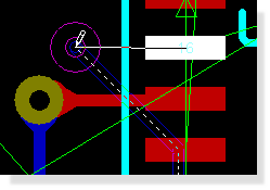
Routing a 45 degree angle
Of course there are many ways we can route the board and personal preference also plays a part. Feel free to experiment with the other connection on the connector, working around the battery holder, using the ratsnest to find a legal destination and then completing the route. The following screenshot is an example of what you might have when you are finished.
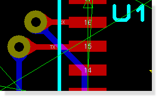
Both tracks fully routed
Basic Auto-Routing
From this point on we’ll use the auto-routing engine to complete placement of the routes. As with the manual tracking the auto-router will obey all the design rules that we configured earlier.
Start by invoking the auto-router from the Tools Menu or from the icon at the top of the application.
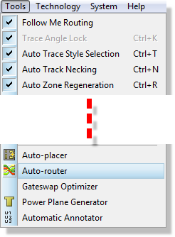
Select the Autorouter from the Tools menu
The resulting dialogue form is reasonably complex but all fields have context sensitive help associated with them. You can also find additional information about the various type of routing pass in the reference manual. For our purposes (and indeed for most boards of small/medium complexity) the defaults are more than adequate. We’ll start by running in ‘fully automated mode’ which should be selected by default so simply hit the begin routing button to complete the remaining connections.
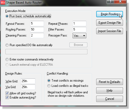
The Autorouter dialogue form
Everything will happen quite quickly from this point onwards but you should see routing progress on the status bar as the engine works towards completion. Once the board is complete there are two immediate points of note :
- The auto-router has preserved those tracks that we placed manually and has not ripped and replaced them whilst working on the rest of the board.
- Once the autorouter has completed a final pass is made to corner the tracks. If you prefer this not to happen you can remove the Recorner Pass option on the dialogue form before invoking the router
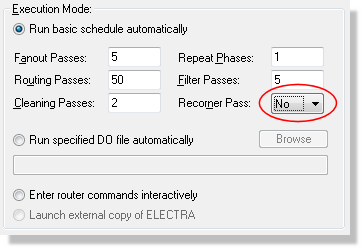
Set the Recorner Pass to be NO
See Also:
Autorouter : Basic Operation (Reference Manual)
Length Matching Routes
Automatic length matching is one of the high speed design features. These, which also include differential pairs, form the Advanced Feature Set and are available in PCB Design Level 2 and upwards.
For high speed signal lines it is common to need to match the lengths of the tracks to ensure that all relevant signals arrive inside the sample and hold time of the receiving chip. While not required for the tutorial design we now have a fully routed board so it is a good opportunity to explain how the feature would be used. The first step is to select the tracks that you wish to length match by holding the CTRL button down and left clicking on each track. We've chosen to do this with two large routes into U1 as shown below
Selecting two tracks for length matching
Next, right click on one of the tracks and select the match route lengths command from the context menu. If successful you will see track segments added in a serpentine pattern to the shorter route in order to match its length with the longer route.
Matched lengths
Full configuration of the added length can be found on the Configure Length Matching command on the Technology Menu or from the context menu.
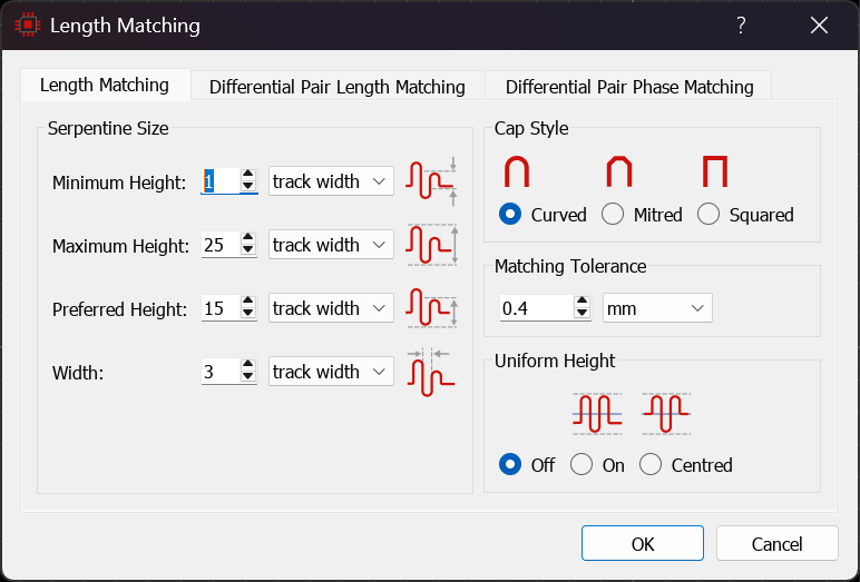
Configuring Length Matching Options.
Other points to note about length matching.
- You can match multiple tracks at the same time (e.g a bus).
- The length of a track is shown on the status bar when it is selected.
- If a track is part of a group that has been length matched the target length is also shown in the status bar when you select the track.
- The pre-production check will test all matched tracks against their target length and warn you if their length has changed.
- If you choose routes with vias the length (depth) of the via is calculated from the thickness values you enter in the layer stackup.
See Also:
Reference Manual : Length Matching Routes
Reference Manual : Differential Pairs
Reference Manual : Manual Routing Examples
The Selection Filter
Now that we have a completed board it’s worth spending a little time looking at the techniques for selecting various object types on different layers.
The Selection filter at the bottom left of the application window is used to determine which objects are available for selection at any given time.
The left most button launches the layers dialogue which allows you to set layer visibility groups and set different colours for different layers.

The green stack icon will determine whether the layer selector is active:
When this is toggled off the selection applies to all layers on the board.

When toggled on the selection applies only to the layer specified in the layer selector

This is an essential technique on a busy multi-layer board as otherwise you'll end up accidentally selecting things on a different layer by mistake.
The other buttons represent different object types (tracks, components, graphics, etc.) and determine whether those object types are selectable. Hover the mouse over an icon for a tooltip description.

If you switch between the different modes of operation (for example from selection mode to track mode to component mode) you will see that the selectable object types will change according to the mode you are in. Whilst these are good defaults for normal operation you can change at any time simply by toggling on or off the layer switch or object type that you do or do not want to be selectable. If you find yourself changing selectable items regularly you can also change the defaults via the System Menu – Set Selection Filter command.
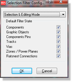
The Layer Selection options
Let’s take a practical example and delete all the traces on the top of the board, except the one we have manually placed. Start by entering Selection Mode and left dragging a selection board around the entire board.
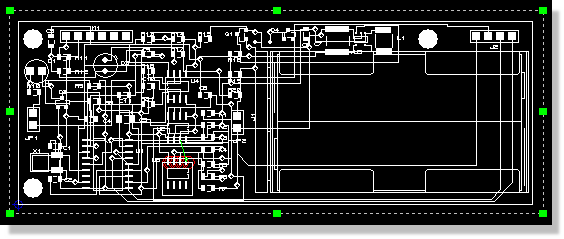
Select the entire board
Next, deselect those objects that we do not want to delete, namely everything apart from tracks and vias. The tagged items will update automatically to provide visual confirmation of what is selected.

Only The tracks will be selected
Now change the layer to be Top Copper on the layer selector and toggle the layer button such that the selection filter applies only to the current layer
Top copper selected
Use the green drag handle at the right of the tagbox to move the selection filter in until it does not encompass the J2 connector.
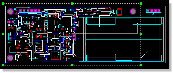
Notice that Only the traces on Top Copper are Selected
Finally, use the icon at the far right of the selection filter to deselect items that are only partially inside the tagbox; in our case this will deselect the track we manually placed from J2, pin 4.

Tag box toggle
We can now simply hit the delete button on the keyboard or right click inside the tagbox and select Block Delete icon to remove all the top copper tracks.
Bear in mind that the selection filter controls what objects are available for selection at any given time. If you ever find that you can’t select an item the first thing to check is whether that object type is enabled for the mode that you are in. Alternatively, simply switch to Selection Mode where all items are selectable.
One other thing can surprise you here. Interacting with any member of an object group expands the selection to the whole group, so if a complete cluster tags when you were expecting a single object, group membership is the reason.
Advanced Auto-Routing
Given that we’ve ripped a lot of partials and removed vias as well we’ve actually made a bit of a mess here. Fortunately, we can fix the situation by simply re-invoking the auto-router and re-placing all our tracks. The router has it’s own clean up phase so it will tidy up all the redundant partial tracks for us as it completes the new routing.
The quickest fix is simply to run the autorouter as we discussed in the previous section and let it re-route the board.
For finer control, the router can also be driven interactively, and we’ll use this section to show in brief some of what that makes possible. These additional capabilities fall into two main categories:
- The ability to route only a specified area or set of connections.
- The ability to control the routing script; i.e. to determine which routing commands are executed and in which order.
Start by invoking the autorouter dialogue form (Tools Menu), switching to Interactive mode and then selecting the Begin Routing button.
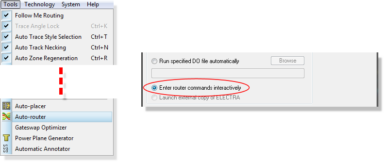
Entering the router interactively
A command window will open at the bottom of the Editing Window, which will allow us to direct the routing progress interactively. Proteus provides a rich command set to control routing, including such things as bend radius for mitering tracks and fanout length and direction from SMT pads. This is fully documented in the reference manual so we will concentrate on some basic practical examples in this tutorial.
There are a couple of important points worth emphasising at this stage:
Any commands entered will action on a set of tagged connections or on the whole board if nothing is highlighted.
Changing the circuit or switching modes will automatically exit the routing interface.
Essentially, what this means is that we can dictate what connections are routed by controlling which items are highlighted.
First of all let’s clean up the loose tracking on bottom copper resulting from our previous rip of the top copper tracks. The basic syntax of most commands is:
<command> <number of passes>
so we can start by typing clean 2 to clean up the superfluous tracking.
Next, lets assume that we want to route all the VCC connections. Select the VCC/VDD=POWER net in the Object Selector and click on the small ‘T’ button above the Object Selector to highlight all the connections on that net. Finally type in ‘route 5’ to route these connections.
Clicking anywhere in the Editing Window will deselect the currently tagged items. When the focus is in the Editing Window you can also use the middle mouse (or keyboard shortcuts) to zoom in and out in the normal way.
Similarly, we can highlight connections on an area of the board and route them independent of the rest of the board. For example, right depress the mouse and drag a selection box around the left half of the board and then type ‘route 10’ to complete open connections in that area.
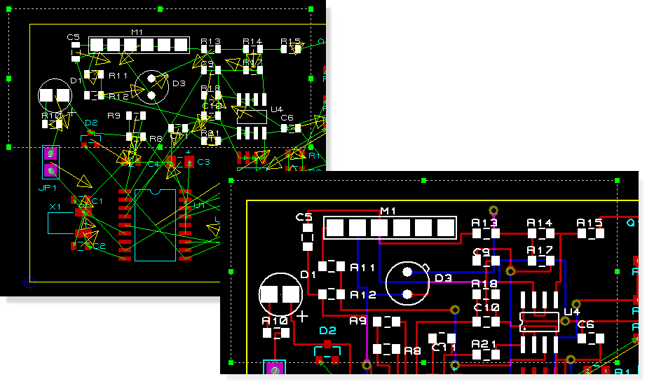
Autorouting an area of the board
You may notice that this has left a couple of ratsnest lines or has not completed all of the connections. We could try to resolve this by issuing clean, filter and more route commands, but for our purposes it’s easier to simply revert back to a ‘whole-board’ scenario and then completing routing. You can do this by left clicking on an empty area of the Editing Window to clear the selection. Typing route 25, followed by clean 2 should see the board completed
Finally, we can reduce trace length by typing recorner diagonal as a finishing touch.
Do note that there is much more flexibility in the command set than that shown in this tutorial, both in the number of commands and in the parameters that control the command actions.
See Also:
Interactive Auto-Routing (Reference Manual)
Command Reference (Reference Manual)
You can exit auto-routing at any time via the ESCAPE button on your keyboard.
Netlists and Design Changes
We have now placed and routed our layout based on the schematic we designed in the tutorial. In practice however, it is very unlikely that we would not be making design changes during the PCB process so we'll devote a little time to examining a typical workflow.
Clearly, we will be editing both the schematic and the layout modules so both need to be open. If the schematic tab is closed you can open it from the application module toolbar at the top of the Proteus application.

Schematic icon on the Application toolbar
Since we will be working with both modules you may want to split them into two frames if you have two monitors. To do this simply drag one of the tabs onto the other monitor. For this documentation, we will assume that both the schematic and the layout are open as tabs inside a single Proteus frame.
Multiple tabs in one frame
Live Netlisting
First, lets delete the J2 connector on the schematic. Switch to the schematic tab, right click and select delete object from the resulting context menu.
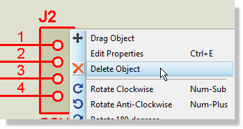
Deleting a component on the schematic
Now switch back to the PCB tab. Note that the J2 part has been dimmed to show that it is not present on the schematic and that the connectivity status shows that we have pending changes (we are out of sync).
Netlist is out of sync
Since the action taken on the schematic removes from the board it requires manual confirmation. We can now either hit undo (CTRL+Z) if we don't like the change or we can click on 'Changes Pending' in the connectivity status to accept the change. When we do this, we'll be presented with a short dialogue to either show all the changes (sometimes not obvious on a dense board) or to simply commit the changes.
Since it's clear what the change is in this case we can simple commit the change and the 'shadow' part will disappear.

Clicking on Changes Pending will remove J2 and correct the netlist
Note that tracks that were connected will also be deleted. If you want instead to delete only the footprint (leaving the connected tracks in place as stubs) then you can do so by directly deleting the package on the layout.
The undo system is still available to revert the changes. Clicking on the UNDO icon (or CTRL+Z) once will bring back the shadow objects and repeating the process a second time will bring back the schematic part and the real PCB footprint.

Undo and Redo icons
If you click on undo while in the layout tab but the undo action applies to the schematic you will be prompted to confirm the operation. In our case, we do want to bring back the connector so accept the prompt to return the PCB to the original state.
This is a simple example of a change which affects objects already placed on the layout. The important thing to remember is that while the netlist is live, you must manually confirm any change which affects the connectivity of objects you have already placed.
Batch Netlisting
If you prefer, live netlisting can be turned off and a more traditional batch mode netlist used. This is controlled from the 'live netlist' toggle on the Tools menu (in the PCB module).
Having turned live netlisting off, let's repeat the same procedure to see the difference. Switch to the schematic tab, delete the connector and then switch back to the PCB tab. This time the connector on the PCB remains present and the connectivity status reports that the layout is locked and out of sync.
Status bar messages when 'out of sync'
This means that we have not loaded the changed netlist and cannot work on the layout until we bring the netlist across. Proteus works with a single database of parts that include schematic components and pcb footprints so - while you can work on the schematic - you cannot work on the PCB until you sync it with the schematic. Click on the connectivity status to unlock the PCB and bring the current netlist across.

This brings us to the same state as we arrived at automatically with live netlisting on. We have a shadow part in Proteus and the connectivity status reports changes pending.
The main difference between live netlisting and batch netlisting is only that you must confirm each netlist load manually in the latter mode. We recommend that live netlisting is used for normal working, although for particularly large designs batch mode may provide a useful tool.
Some functionality will require a live netlist and so if you are working in batch mode you may find menu commands disabled until such time as you bring the netlist back in and sync.
See Also:
Netlist Features (Reference Manual)
Annotation
Annotation changes from schematic to layout or from layout to schematic are also a common editing operation when both modules are in use.
Schematic to PCB
Annotation changes made in the schematic will automatically be reflected in the PCB when live netlisting is on and will require unlocking when live netlisting is off. The Global Annotator on the Tools Menu on the schematic can automate this task.
PCB to Schematic
You can re-annotate the board either manually (editing the part reference labels) or globally from the automatic annotator command on the tools menu.
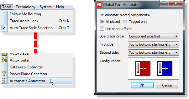
Launching the Automatic Annotator
When live netlisting is on, this will automatically reflect to the schematic. With live netlisting off, the schematic will update and the layout will then lock as the netlist has changed and needs to be manually passed through to the layout.
General Netlisting Rules
There are several important rules of thumb to understand about netlisting in Proteus.
When live netlisting is on, a change that adds connectivity will happen automatically (e.g. adding a wire on the schematic will add a ratsnest on the layout). If you make a change that removes connectivity the layout will show the change by dimming the deleted objects and you will need to manual confirm the operation.
When live netlisting is off (batch netlisting) any and all changes to the netlist will require you to unlock and apply the netlist before you can continue working on the layout.
Clicking on changes pending to remove footprints that have been deleted on the schematic will also remove associated tracks. If you want to remove footprint only and leave the tracks simply delete the part on the layout (rather than the schematic).
Dimmed objects are visual placeholders only - they do not exist on the board. Best practice is always to click on changes pending on the connectivity status and to arrange the layout to conform to the schematic.
Imported projects (from older versions) will always start with live netlisting off as there is no way to tell whether they are in sync. By contrast, new projects will always start with live netlisting on. In either case you can switch according to preference from the live netlisting toggle on the Tools menu in the PCB layout module.
Power Planes and Slots
If you switch back to the layout tab we will continue the layout phase of the project. To minimise track impedance we are going to place a power plane covering the entire board.
Placing Power Planes
This is actually the easiest type of power plane to place. Start by invoking the power plane generator command from the Tools Menu
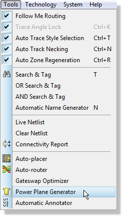
Opening the Power Plane Generator from the Tools menu
From the resulting dialogue form select the GND=POWER net, keeping the layer as bottom copper and setting the boundary style to be T10. This is the trace style in which the inner and outer boundaries of the zone are drawn and also determines the thinnest section of copper by which the power plane can make a connection. Setting this larger will prevent the copper flowing through small gaps (e.g. between pins) but making it smaller means that connectivity may be made only by thin sections of copper.
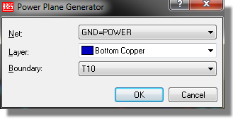
Power Plane Generator Dialogue form
After you exit the dialogue form you should see that the power plane is generated across the entire board.
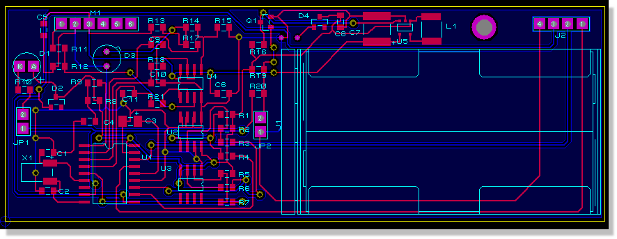
Power Plane has flooded the entire layer
The clearance from the zone to the board edge is defined by the Edge/Slot design rule. We can change this via the Design Rule Manager on the Technology and the zone will re-generate to the new clearance when we have finished.
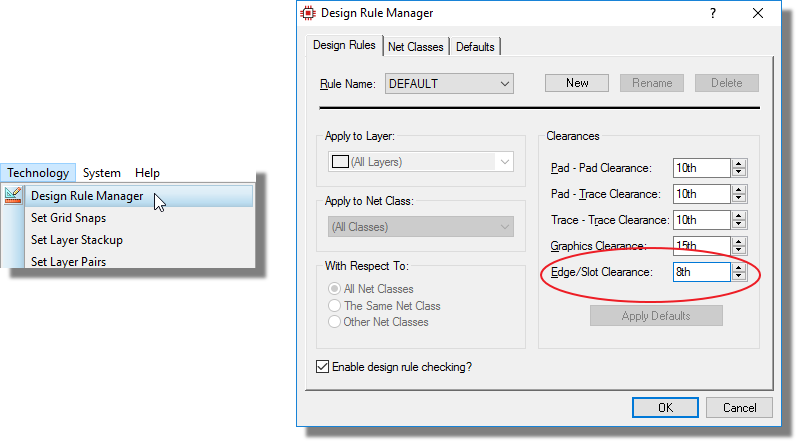
Since you can set a new design rule per layer it is possible to have different clearance rules for power planes on different layers
On multi-layer boards where you want to specify one or more internal layers as plane layers you should do so via the layer stackup manager.
Stitching Zones
In Proteus you can auto stitch / shield a power plane. This is done by right clicking on the edge of a power plane and select the relevant option:
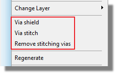
Stitching is fully explained in the Reference Manual: Stitching and Shielding.
Split Planes & Zone Inspector
You can place split or partial planes in zone mode at the left hand side. Then you either drag a box to make a rectangular plane or left click consecutively to make a polygonal plane.

Note that in Zone mode the parts bin will show you a list of zones placed on different layers of the board. Double clicking on an entry will tag a navigate to the plane on the layout.
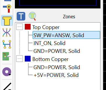
For a full analysis of zones on the board click on the Zone Inspector icon above the parts bin in Zone mode or launch directly from the Tools Menu.
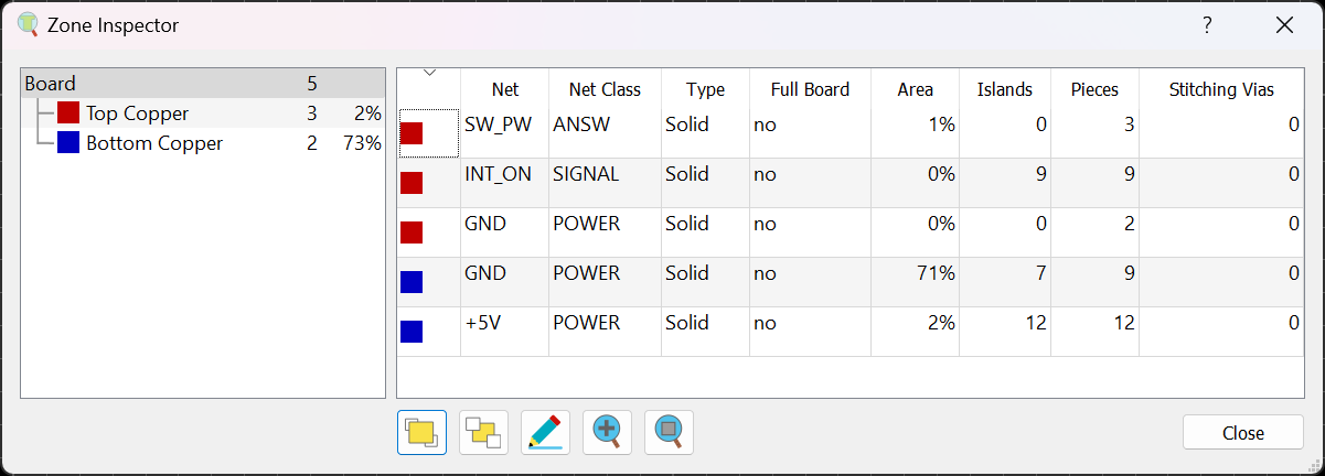
Nesting and Islands
There are several additional configuration options available to us now that we have placed the zone. Editing a zone is slightly different from most other objects in that you must right click on the border of the zone (to avoid continuous unwanted selections).
You can also edit a zone from inside Zone Inspector as discussed above.
Firstly, check the selection filter and make sure that the zone object type is selectable (or switch to selection mode).

Zone icon in the Selection Filter
Next, zoom in and move the mouse over the edge of the zone, right clicking the mouse when the zone is shown as active under the mouse. Select the Edit Properties from the resulting context menu.
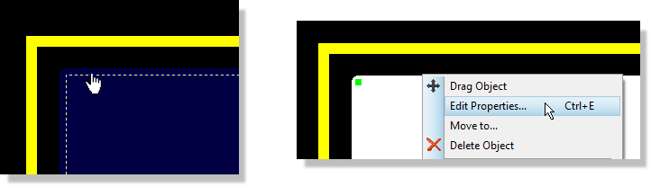
Right click on the edge of a zone to edit its options
The main options of interest are towards the bottom of the dialogue form and are explained below:
Relieve Pins
When checked pins on the same net as the zone will have thermal relief applied to them; the thickness of the thermal relief is determined by the Relief field of the dialogue form.
The software will prevent you from using a relief track style that is larger than the boundary style thickness; this is to protect against the reliefs 'sticking out' of the boundary.
The topology of the relief stems on a particular pad can be changed to a diagonal 'X' by editing the pad itself after placement. This is sometimes useful to maximise contact with a zone.
This option should almost always be left in it’s default checked state.
Exclude Tracking
If this option is checked, the zone will treat tracks on its own net as obstacles. Otherwise the zone flows over such tracking, effectively ignoring it. Tracks on other nets, or loose pieces of track on no net are always treated as obstacles.
This option is normally left unchecked.
Suppress Islands
An island is defined as a block of copper or zone area in which no valid connections can be made. When checked, Proteus will remove all such blocks from the board, leaving only areas of copper with connections.
Allow Nesting
It is quite common, particularly with larger boards, that the flow of a zone will encounter an obstacle through which it cannot pass. When checked, the zone will jump over the obstacle and continue flowing across the board.
This is a very useful option for example on busy boards or where you want to connect a pad where the topology of the board makes it impossible for a single zone flow to get through.
Given our relatively simple board, the default options are ideal for our purposes. Selecting the nesting option will have no effect for example as there are no inner boundaries on the board. However, if you want to experiment you should find that if you uncheck 'suppress islands' option, the resulting zone populates far more of the board that in our initial configuration.
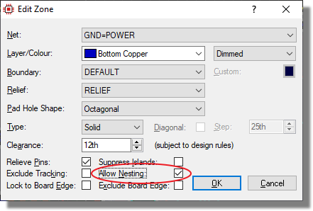
We have covered only the basics of power plane functionality here relevant to our current design. For more information, including split planes, zone keepouts, stitching and bridge tracking please see the power planes section of the reference manual.
See Also:
Power Planes Examples (Reference Manual)
Using Power Planes (Reference Manual)
Plane Layers (Reference Manual)
Via Stitching and Via Shielding of Power Planes
Zone Inspector (Reference Manual)
Slots
To complete the layout of the board we need to return to our temperature/humidity sensor (U3). In order to make accurate measurements, we want a thermal cutout around this part, ensuring that the temperature we are measuring is actually the environmental temperature and not conducted heat from the PCB.
You may remember that we placed a keepout area around this part to prevent the autorouter from placing tracks through the area we want to cut out. Start by zooming in around U3 and removing the keepout. You’ll need to either switch to Selection Mode or to change the selection filter such that you can select 2D Graphics
Deleting a Keepout area
While we are here we might as well move across and deal with the other keepout, the one around the crystal. That one needs a little more care. We made it a member of the crystal group earlier, and deleting any member of a group deletes the entire group, so right clicking on the keepout and choosing Delete Object would take the crystal and its capacitors with it.
Right click on the keepout graphic, select Ungroup Objects, and then delete the graphic on its own. Ungrouping dissolves the whole group, so the crystal and its capacitors are loose objects again afterwards. Group them once more if you want to keep the block travelling together for the rest of the design.
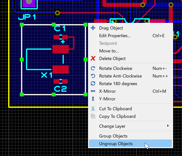
Ungroup Objects on the keepout context menu, which must be used before the keepout graphic can be deleted on its own
Returning to U3, we now need to outline the cutout region. In the layout editor this works much the same as placing anything else. We select the 2D Graphic Line, choose the slot layer and then place three lines to form a ‘U’ shaped cutout.
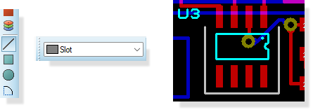
Placing a slot on the SLOT layer
Finally, we can thicken these three lines to something more appropriate as follows:
Enter selection mode, hold the CTRL button down on the keypad and left click once on each line. This will select all three lines
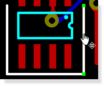
Selected items are white
Right click on any line and select Edit Properties from the resulting context menu.
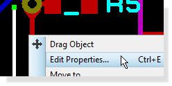
Uncheck the Follow Global checkbox, change the width to be 20th and then apply to all tagged graphics.
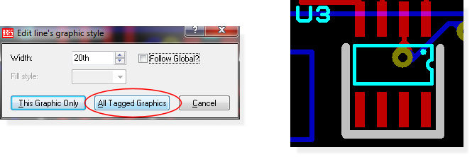
Changing multiple objects at once
Thickening the lines moves the cut edge closer to the pads of U3, and we turned the edge clearance test off inside this area when we set up the design room, so nothing is going to warn us if the slot ends up too close. It is worth taking a measurement before we move on. Select Measure Mode, left click on the nearest U3 pad, left click on the slot line beside it and select Nearby Closest Points to read the edge to edge gap. If it is tighter than your fabricator is happy with, click Swap Direction so that the arrow tip is on the slot graphic and then move the line out to the distance you want.
3D Visualisation
Now that the board is now routed and ready for production we first want to examine it in 3D in order that we can properly preview how it will look in real life and possibly make final design alterations prior to prototyping. Start by invoking the 3D Visualisation Engine from the module toolbar at the top of the application

3D Viewer icon
This will open and load the 3D view of the board in a separate tab. As with any tab, you can drag onto a separate frame if you want to look at both the 2D layout and the 3D view simultaneously.
Basic Navigation
The first thing we can do is view the board from different preset angles. Five preset views are supplied: top view, front view, back view, left view and right view and these are accessible via any of the following methods:
- Menu options on the View menu in the 3D Viewer
- From the navigation toolbar at the bottom of the 3D Viewer
- From keyboard shortcuts F8 through F12 whilst in the 3D Viewer.

Now that we can look at the board from a number of angles the next thing is to be able to look at it at a specific zoom level. Again, there are numerous ways to zoom in and out of the board:
- Roll the middle mouse wheel in and out (recommended)
- Menu options on the View menu
- From the icons on the Navigation Menu
- From keyboard shortcuts F6 (zoom in) and F7 (zoom out)
Experiment now with custom zoom levels and different preset views – whilst it is pretty subjective we envisage most users changing views via the navigation toolbar or keyboard shortcuts and using the middle mouse wheel to zoom in and out.
Bareboard View and Height Clearances
For inspection of resist and hole depth it is often useful to view the board without components. Selecting the bareboard view will remove all the physical components from the board.

Show Components icon
By contrast, if you need to fit the PCB into a chassis and wish to check height clearances you can enable the height boundary box via the icon at the bottom of the display

Casing icon
Specification of the height takes place from the Dimensions command on the Settings menu of the viewer. This will default to the values defined in the layer stackup.
The Dimensions dialogue in the 3D Viewer, where the height boundary box is specified
Custom Views
The next logical step is to be able to customise the view. This works conceptually by ‘attaching’ the mouse to the camera such that as you move the mouse the camera moves to the area of the board that you are interested in. You can invoke the Navigation mode either from the View menu, the crosshairs icon on the Navigation toolbar or simply by clicking the left mouse button.
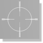
3D Mouse cursor
You will know as soon as you are in Navigation mode as a crosshair cursor will appear over the mouse and your view of the board will change as you move the mouse. Using this together with the middle mouse wheel zoom will allow you to both ‘fly pass’ the board and to easily zoom in to closely examine a particular area of the board. Exiting navigation mode is as simple as right clicking the mouse.
For example, if we start in Front View (use the F9 keyboard shortcut) and we want to examine the resistors on the right we might proceed as follows:
1) Left click the mouse to enter navigation mode.
2) Move the mouse over the resistors.
3) Roll the middle mouse button to zoom in as required.
4) Right click the mouse to exit navigation mode.
The final necessary piece to completely customise the view is to allow users to spin or ‘orbit’ the board. This is done in navigation mode by holding down the left mouse button and moving the mouse. Essentially this will spin the board as you move the mouse – when you release the mouse button the camera will follow the mouse around the current view of the board as normal. Try this now, experimenting with different views of components on the board.
Remember that, if you are struggling to get the view you want you can use the keyboard shortcuts or navigation toolbar to return to one of the preset views. You should find however, that with only a little practise you become quite proficient at navigation.
To summarise:
- Left click enters navigation mode.
- Camera follows mouse around the board in navigation mode.
- Using the middle mouse wheel (or shortcut keys) allows you to zoom as you move the camera.
- Left depressing the mouse in navigation mode allows you to spin/orbit the entire board.
- Right click of the mouse exits navigation mode.
3D Models (STEP/IGES)
Each footprint on the layout can also have an associated 3D model. Normally, these are either STEP Files (for large or complex parts) or scripted geometric models (for simple passives).
In the case of STEP or IGES files, the procedure is:
1) Download the file from the internet or otherwise source the 3D model. There are many sites available, with www.3dcontentcentral.com being amongst the most popular.
2) Save the file into the MCAD directory of your Proteus installation.
3) Right click on the footprint and select Make Package, and then click on the 3D Mechanical Model tab.
4) Type the name of the STEP file and then the rotation and offset required to align the STEP file with the pads on the board.
For geometric models, the difference is basically that you describe the part in terms of size and shape via a simple scripting language. This is covered in the reference manual.
See Also
Live Update
Like any other module in Proteus, the 3D Viewer will update live as changes are made to the PCB layout module. In practice, the usefulness of this will depend very much on the power of your machine (number of cores, memory, etc.) and the complexity of the board.
On a board of modest complexity and a modern computer the redraw time is not significant and - particularly on split frames - is very useful for movement and positioning.
More information on 3D visualisation, including creating your own 3D models, exporting 3D STEP files for MCAD import, customisations and applying 3D data to legacy designs, can be found in the 3D Viewer section of the online reference manual.
The 3D export can also be generated as part of an output job; see the Output Job Manager section at the end of the next chapter.
Board Output Options
Last, but by no means least, we come to the crucial business of turning the design on screen into the files and drawings that other people need. There are two ways of going about this in Proteus and it is worth understanding the difference before we start.
The first is ad-hoc output: you invoke a single command, configure the dialogue and generate one thing. Printing a layout and running a one-off set of Gerber files both work this way, and it is the right approach when you want one specific output right now. We will use it for both in the sections that follow, because the per-format dialogues are where the real configuration lives and we need to understand them.
The second is managed output: you define a job profile once, listing every output the project needs and how each one is configured, and then generate the whole manufacturing pack with a single click. That is the Output Job Manager and we will come to it at the end of the chapter, once the individual dialogues make sense.
Printing
We will deal here firstly with printing to an ordinary Windows printer device. With a layout loaded, invoke the Print Layout command from the Output menu. Device selection sits inside the dialogue itself, so there is no separate setup step: pick the printer you want from the dialogue and configure it there. The options offered by the printer will depend on your version of Windows and on the printer driver, so consult the Windows and driver documentation for those.
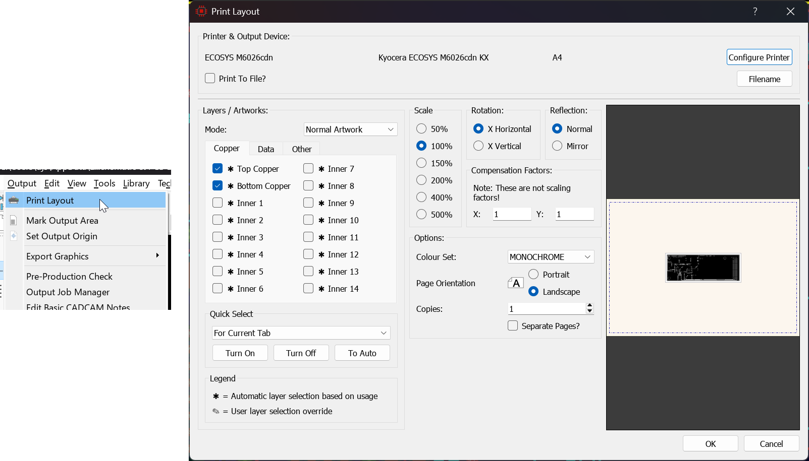
The Print Layout dialogue, with printer selection and layer options in one place
The dialogue forms offer a number of controls, all of which have context sensitive help associated with them (context sensitive help on dialogue forms is accessed with a ‘point and shoot’ mechanism via the ‘?’ key at the top right of the dialogue form). The default settings should do for getting something and you commence output generation by clicking on OK. Output can be aborted by pressing ESC, although there may be a short delay before everything stops whilst Proteus and your printer/plotter empty their buffers.
Full details of the printing options may be found under the chapter Hard Copy Generation in the reference manual.
Proteus will remember your printer settings and maintain them independently of your printer settings for other applications. This means that you can configure a default set of printer options solely for use with the Proteus application.
Printing is not something that can be added to an output job, since it needs a physical device at the other end. A PDF of the layout can be, however, so if what you actually want is a shareable drawing of the board rather than paper, add a PDF Document task to the Output Job Manager profile we set up at the end of this chapter and it will be produced along with everything else.
See Also:
Output for Manufacture
Pick and Place
ARES has the ability to output a fully configurable Pick and Place file. The configuration is mostly a matter of matching your assembly house: the combo boxes let you set the order of the columns and you can rename each column heading so that the insertion machine recognises it. For more information please see the reference manual here.
Default column names follow the column order automatically, but custom names do not. If you have renamed any of the headings and then change the column order, you must re-order the names by hand to match. Check the preview at the bottom of the dialogue and confirm that each heading still sits above the right data.
The Pick and Place file can also be generated as part of an output job; see the Output Job Manager section, where we add it to the pack alongside the Gerber output.
Gerber
Proteus provides three main output options for board manufacture:
- Traditional RS274X Gerber/Excellon.
- Gerber X2.
- ODB++ Manufacturing Output.
From a user interface perspective all options are very similar but from a manufacturing perspective, Gerber X2 provides far more information than the older Gerber formats. Examples include:
- Inclusion of the connectivity information (IPC-D-356A netlist) with the output fileset.
- Independent Gerber files for each drill range and plated/unplated status.
- File and object attributes automatically applied (for example, a fiducial is identified explicitly as a fiducial).
- Full backwards compatibility with standard RS274X. In addition to the Proteus Gerber Viewer, files will load into any third party reader of your choice.
- Automatic inclusion of both Top and Bottom assembly drawings.
All of this means that when viewing the output fileset from Gerber X2 the verification process is simpler and more complete. However, traditional Gerber/Excellon output is still widely used in manufacture and would be sufficient for most purposes.
Regardless of your option the basic procedure is the same. Gerber and Gerber X2 are both produced by the Generate Gerber/Excellon Files command on the Output menu, with ODB++ produced by the Generate ODB++ Database command alongside it. Note that ODB++ is not one of the output job task types, so unlike Gerber it cannot be batched: if your fabricator asks for ODB++ you will need to run that command separately. When you invoke either of the output options you will most likely be prompted to run a pre-production check. This runs an automatic checklist to test for some common design errors and will report either a pass or a fail.
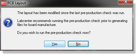
The Pre-production check (PPC) prompt
If your pre-production check reports errors we strongly recommend that you resolve them before proceeding to the manufacturing output dialogue. Please also note that pre-production check is an aid to the designer in quality assurance but not a guarantee; manual inspection of the layout is recommended and a prototype should always be made and tested before mass production.
More information on the Pre-production Check can be found in the Output for Manufacture section of the reference manual (Help Menu).
Assuming a pass you will then be provided with the manufacturing output dialogue form
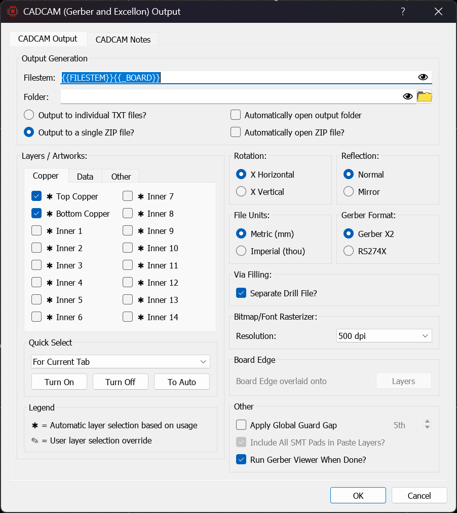
The Gerber / Excellon Output dialogue form
The options in the top section of the dialogue form are fairly self-explanatory. The field codes in Proteus are placeholders for common information that may change between projects or between output generation but has the same meaning regardless. You can get a list of field codes for use by right clicking on the edit fields or you can simply type paths and names in manually if you prefer. You'll find more information in the Output for Manufacture section of the main reference manual.
Some points of note regarding the rest of the configuration options:
The software attempts to populate the layer set with those layers used on the layout but this should always be verified. One of the most common problems with manufacture occurs when the manufacturer is not supplied with the full board information.
The Apply Global Guard Gap option will set the expansion of the resist plot around pads and vias to the distance specified when this option is checked. This will take effect on all pads and vias except those which have been manually altered on the layout. Some board manufacturers prefer to create the resist plot in house and this option could then be used to remove any resist expansion pre-manufacture. Unless otherwise directed we recommend that you leave this option unchecked.
The Bitmap/Font Rasterizer option controls the thickness of trace used to render bitmaps and true type fonts. The higher the resolution the better tonality of the resulting bitmaps but the larger the files. It is also possible that some manufacturers have a minimum width requirement and in such cases it may be necessary to reduce the DPI settings to conform with this. Generally speaking however, the default settings are fine.
The option at the bottom left allows you to automatically load your output into either the Labcenter Gerber Viewer (Gerber/Excellon output) or the Valor ODB++ Viewer (ODB++ output). This is useful if you want to verify the output fileset before passing to your manufacturing house.
If you intend to panelise the board you should use the Gerber X2 output in the Generate Gerber/Excellon Files command, then close the project, open the gerber module and import your CADCAM files, selecting Panelisation Mode from the resulting dialogue form. Panelisation is only available with Gerber X2 output; you cannot create panels from RS274X Gerber. Note that the panelising itself happens in the separate gerber module rather than in an output job, although the Gerber X2 files that feed it can perfectly well be produced by one.
See Also:
Panelisation (Reference Manual)
Finally, the Notes tab allows us to insert any relevant information or special considerations for the manufacturer. You can also choose to include your manufacturing notes from the Project Notes module if you prefer.
See Also:
Reference Manual - Manufacturing Report
Project Notes : PCB Specification Notes.
Having configured the necessary option we can generate the files and send for manufacture. That completes the ad-hoc route; what follows is how to batch the same output, configured exactly as we have just configured it here, so that the whole pack comes out of a single command.
The Output Job Manager
Our board needs more than one file to reach manufacture. The Gerber and drill set goes to the fabricator, the Pick and Place file goes to the assembly house, and if we revise the design we will need both again. Running each command by hand every time is where mistakes creep in: a file gets missed, or a setting that was adjusted for one output is forgotten for the next. The Output Job Manager solves this by letting us describe the whole set once and then generate it in one operation.
The command sits on the Output menu, between Pre-Production Check and Edit Basic CADCAM Notes.
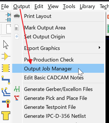
The Output Job Manager command on the Output menu
The first time you open it there are no profiles, so click New and give the profile a name. We will call ours Manufacturing.
Next set the job folder, which is the root beneath which everything the job produces is written. Type:
{{DIRECTORY}}\Output
The double braces are field codes, placeholders that are resolved when the job runs. {{DIRECTORY}} is the project directory, so the output lands in an Output folder beside the project wherever the project happens to live. The eye icon beside the field toggles between the expression and the path it currently resolves to, which is worth a glance before you generate anything.
Now add the two tasks this board actually needs. For each one we set a sub-folder and a filestem:
1) Add a Gerber task. Set the sub-folder to Gerber and the filestem to {{FILESTEM}}{{_BOARD}}.
2) Add a Pick and Place task. Set the sub-folder to Assembly and use the same filestem.
{{FILESTEM}} is the project name without its extension. {{_BOARD}} is the conditional form of {{BOARD}}: the leading underscore is included only when the board name resolves to something, so a single board project such as ours produces a clean name with no trailing underscore, while a multi-board project gets one distinctly named file per board.
Each task also has a Configure button, and this is where the earlier part of the chapter pays off. Configure on the Gerber task opens the same manufacturing output dialogue we have just worked through, and Configure on the Pick and Place task opens the same column settings. The choices you make are stored in the profile rather than in the project, so they are applied identically every time the job runs. There is no need to fill in a folder or filestem inside those dialogues; the job manager overrides them with the paths we have just defined.
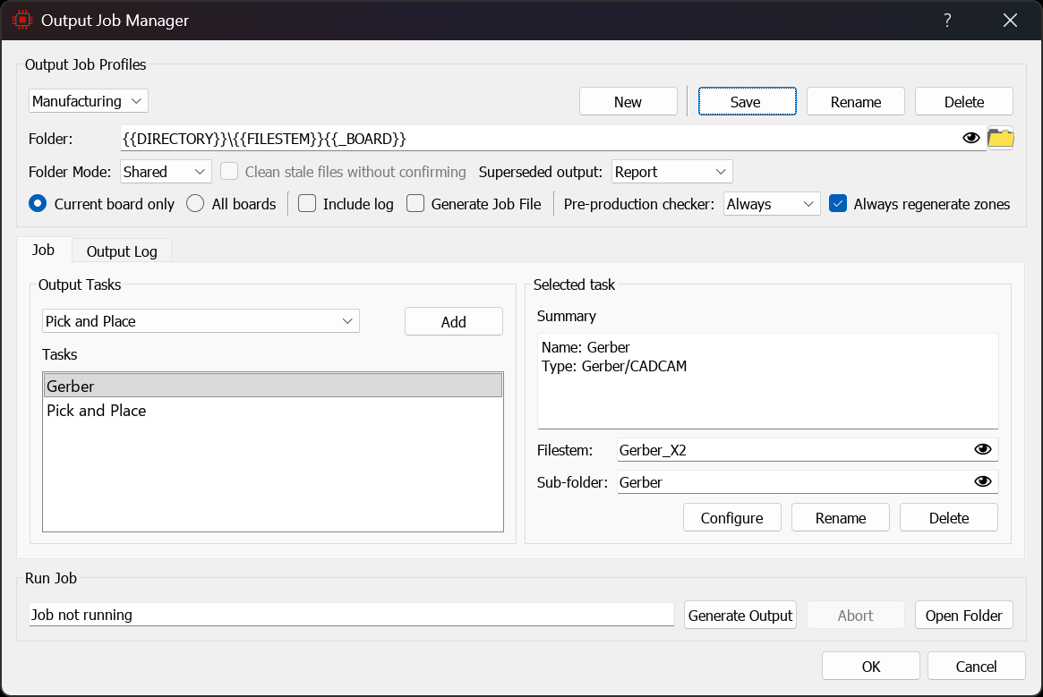
The Manufacturing profile with a Gerber task and a Pick and Place task, each with its own sub-folder and field code filestem
Two of the job level settings above the task list are worth pausing on.
Always Regenerate Zones is on by default and should stay that way. We poured a GND plane across the whole of bottom copper two chapters ago, and a zone fill that is out of date will be written to the Gerber files exactly as stale as it appears on screen. With this option checked, Proteus rebuilds every zone before a single file is produced.
The pre-production checker dropdown offers As needed, Always and Never. This is the same checker that prompted us when we generated the Gerber files by hand, except that here it runs automatically before every pack without showing its dialogue, and any failures are recorded in the output log for us to review alongside the generated files. Leave it on Always. Never is documented as not recommended, and with good reason: an unconnected net is a great deal cheaper to find now than after the boards come back.
Click Save. The profile is written as a .poprof file in the templates directory, so it persists between sessions and can be copied to a colleague's machine. Because the paths are field codes rather than fixed directories, a shared profile resolves correctly on whatever machine and project it is used with.
Finally, click Generate Output. The dialogue switches to the Output Log tab and reports each stage as it happens: the output folder is prepared, the zones are regenerated, the pre-production checker runs and then each task executes in list order. When it finishes, the complete pack is sitting in one folder tree, produced by a single click.
The Output Log tab after a successful run, listing each task and the files it produced
Add {{REV}} to the job folder path, for example {{DIRECTORY}}\Output\{{REV}}, and every revision of the design gets its own output directory automatically. The revision comes from Edit Design Properties in the schematic module, so bumping that one field is all it takes to keep a clean archive of every fileset you have released.
See Also:
Output Jobs (Reference Manual)
Field Codes (Reference Manual)
Where Next
That is the board finished. Starting from the schematic we brought across a live netlist, defined a board edge and a layer stackup, placed and positioned the components, set the design rules and net classes, routed the board both by hand and with the autorouter, took a design change back through from the schematic, poured a ground plane, cut a thermal slot, checked the result in 3D and produced the manufacturing pack. From here, one click regenerates that pack whenever the design changes.
If you have worked through the exercises you now have enough of the software to start a board of your own, and that is much the best way to consolidate it. There are two obvious places to go next.
- The advanced PCB tutorial works a more demanding board and covers differential pairs, length matching in depth, via stitching, fiducials, DRC rooms and the Project Notes module. It is available from the Help menu alongside this one.
- The reference manual covers every feature in full. Remember too that each dialogue in Proteus has its own context sensitive help, reached from the question mark button at its top right, which is usually the quickest way to answer a question about one specific field.
The appendix that follows covers creating your own footprints, which you will need sooner or later even with the libraries and the part importer to hand.
APPENDIX: Creating New Packages
Proteus comes pre-supplied with a large quantity of footprints, and we have seen previously how to select and place these parts on to a layout. However, it may be necessary at times to create your own custom footprints or symbols – also a simple task with Proteus – and this process is detailed below.
While the following topics are a detailed explanation of how to create component parts in Proteus, in practice this should almost never be necessary. In addition to the many installed libraries the universal part importer provides support for almost all third party part vendors (Ultra-Librarian, Samacsys, SnapEDA, etc.). If the part doesn't exist in Proteus itself the next step is to search for and then import it directly from a third party vendor. This is discussed in some detail in the importer help file and shown on our Youtube Channel.
There is one more route worth knowing about. ProPilot, the AI assistant in the schematic capture module, can generate a schematic symbol and a matching footprint from datasheet screenshots. It is not a substitute for reading the land pattern drawing, so always check the generated footprint against the datasheet dimensions before you commit it to a library. ProPilot is available in the schematic module rather than here in the layout module.
See Also:
Library Part Creation with ProPilot
Drawing the Footprint
In our example, we will create a SQFP44 footprint with 0.8mm pitch and 12mm width. You may also wish to refer to the more advanced video tutorials linked below:
Creating Button Pads / Membrane Touchpads with custom paste and resist.
Creating QFN Parts with Thermal Pads and patterned Paste Mask
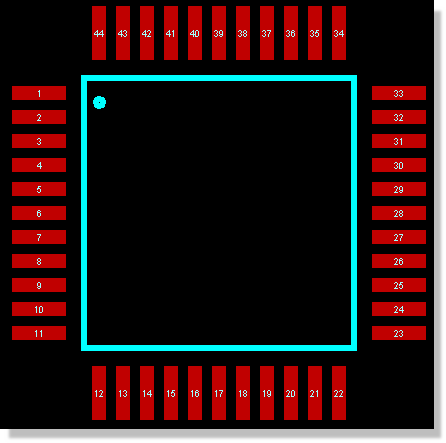
Finished SQFP44
Start by selecting rectangular SMT mode. We want a pad 0.5mm by 1.8mm that should already exist as M0.5x1.8.
The Pad used in the M0.5x1.8
If the pad style does not exist you can easily create it as discussed earlier in the tutorial (Click on the ‘C’ button above the Object Selector).
Make sure that the Layer Selector is on Top Copper and place one of the pads in the usual way. Right click to cancel placement immediately after placing a single pad and then left click on the pad to highlight it. With the pad highlighted, go to the Edit Menu and select the replicate command, just as we did when placing the mounting holes. Alternatively you can right click on the pad and select replicate from the resulting context menu.
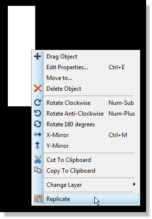
Right click and select the replicate command
The replicate command will action on tagged objects so you should ensure that you have only the placed pad highlighted before invoking this command.
Do not group the primitives of a footprint as you build it. Replicate is one of the commands that is not group aware, so it acts on the individual objects you have selected rather than expanding to the rest of the group, and the whole of this appendix leans on Replicate. Object groups are for arranging objects on a finished layout, not for constructing a package.
There are 11 pads on each side of the footprint so we need to replicate 10 times with an X-Step of 0.8mm as per the following screenshot.
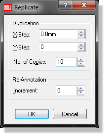
Replicate Dialogue
Note that you need to include the units of either millimetres (mm) or Thou (th) when entering values in to the X/Y-step fields.
This will give us a single row of pads of the correct pitch. If you would like to confirm it, switch to Measure Mode, click on two adjacent pads and select Original Points to read the centre to centre pitch. The next step is to duplicate this row of pads to form the bottom of the footprint.
Start by right dragging a tagbox around the entire row of pads and then go to the Edit menu and select replicate. This time we want only one copy, 12mm down (or up) from the current row. Use negative co-ordinates if you want the duplicated row beneath the current one or positive co-ordinates if you want it above.
We now need to repeat the process with the other two rows. Drag a tagbox around a full row, right click inside the tagbox and select Block Copy from the resulting context menu.
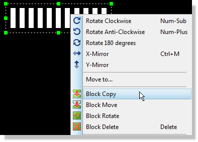
Block copy will copy everything inside the tag box
Move the mouse and drag the copy to a free area, left clicking to place and then right clicking to exit copy mode. Now, drag a tagbox around the row, right click and select the Block Rotate option, specifying a 90 degree rotation to align the pads correctly.
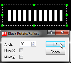
Block rotation of 90 degrees
In order to position this row of pads correctly it’s best to first set place a marker on the location we want to move the row of pads to. For this footprint the centre of the top pad on the left hand side is 2mm below and 2mm to the left of the centre of the left hand most pad on the top row. This gives us enough information to accurately position the row.
Select marker mode in preparation and then move the mouse over the left hand most pad on the top row until it is encircled. You’ll want to be on a fairly precise snap setting for this (e.g. 0.5mm or F2 shortcut key).
Make sure the pad is encircled
If you find your snap settings in thou you need to switch to Metric mode, either by hitting the ‘M’ key on the keyboard or via the Metric option on the View Menu.
Now, hit the ‘O’ key on the keyboard to set a false origin at this location and then invoke the Goto Position command from the View Menu (CTRL+G).
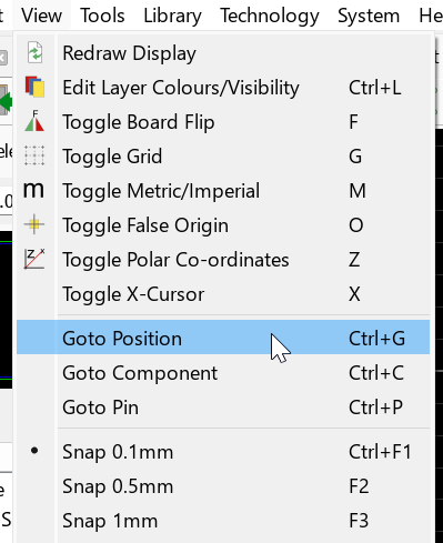
Type in –2mm in both the X and the Y co-ordinate fields (i.e. down and left) and make sure that the offset is relative to the current origin. Select OK and click the mouse twice to place the marker at this location.
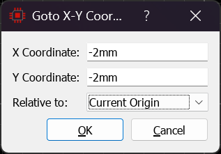
OK will take the mouse to the specified location
The marker we have placed will serve for now as the location we want to centre the top most pad of our third row. Simply draw a tagbox around the row, left depress the mouse inside the selection box and drag into position. You will almost certainly need to use the zoom commands (F6,F7 or the middle mouse wheel) and possibly also adjust the snap setting (CTRL+F1) to get accurate positioning.
Moving the centre of a pad on to the marker
Having placed the row of pads right click on the marker and delete it – we’ll come back to marker placement later on. The final stage of pad placement is to replicate the newly placed row of pads onto the right hand side. As before, draw a selection box around the row of pads and use the replicate command with an X offset of 12mm to duplicate the row.
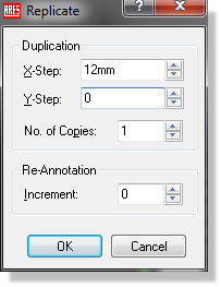
Adding the silkscreen graphics is now straightforward. Select the 2D Graphics Line icon, make sure the Layer Selector is on top silk and place four lines along the inside edges of the pads to form a box. You’ll find this much easier to do if you change the snap settings upwards (e.g. F2).
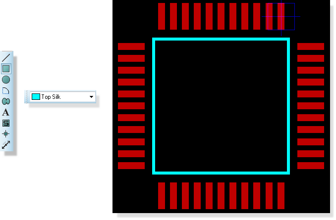
Placing the Top Silk area
The next job we have is to number the pads. Start by invoking the Automatic Name Generator from the Tools Menu (default key mapping ‘N’). We don’t need to enter anything in the string field here; simply leave the defaults and click on the pads consecutively to number them, Number 1 is the top pad on the left hand row.
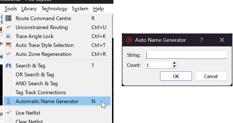
The Automatic Name Generator
Remember to hit the escape key on your keyboard when you have finished numbering pin 44 to exit assignment mode.
It’s common to place a small dot beside pin one and you can do this via the 2D Graphics circle icon. Make sure that the Layer Selector is on Top Silk and turn the snap setting down to minimum (CTRL+F1) to achieve finer control over the size.
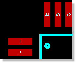
Place a small dot where Pin 1 is
The final step is to specify where we want the origin of the device to be (for placement purposes) and where we want the silkscreen graphics for the package reference to appear. Both of these are done with markers.
Select marker mode and make sure that ORIGIN marker is highlighted in the Object Selector. You’ll recall that we used this as a reference point earlier but it’s real job is to specify the origin of the component for placement and rotation. This is really a decision for the user but typically the origin is either pin 1 or the centre of the component. For simplicity here, we will place the origin on pin 1; left click to begin placement, move the mouse over the centre of pin 1 and left click again to commit the origin marker.
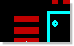
Origin marker placed
Now, change the marker type to be REFERENCE in the Object Selector. The Reference marker dictates where the component reference (e.g. U1, R12, C3) is placed by the software relative to the component. Again, this is very subjective but we’ll set it above and slightly to the left of the part.
Reference marker placed
Having completed the layout of the footprint, we can now move on to the (far simpler) process of packaging the part into the libraries.
Circular Pad Placement
The replicate command is dynamic based on whether you are in cartesian co-ordinates or polar co-ordinates (View Menu Toggle). If you needed to place pads in a circular shape you would:
- Select Polar mode (View Menu).

- Place a False Origin ('O' shortcut key).

- Orient your first pad and place at radius distance from (false) origin.

- Right click on the pad, select replicate comm and and specify angle (e.g. 20) and number (e.g. 17) to complete the circle.

Packaging the Footprint
Drag a selection box around the entire footprint and then select the Make Package command from the Library Menu.
Launch 'Make Package' from the Library menu
The first screen is fairly self-explanatory and similar to that we’ve seen in the schematic application. Note that the package description is searchable when we are browsing for footprints so a little effort to make this as descriptive as possible is worthwhile. You will also want to create the part in the USERPKG library which is the default library supplied for user footprints. For our purposes, we’ll call this package TESTPKG and give it some basic entries.
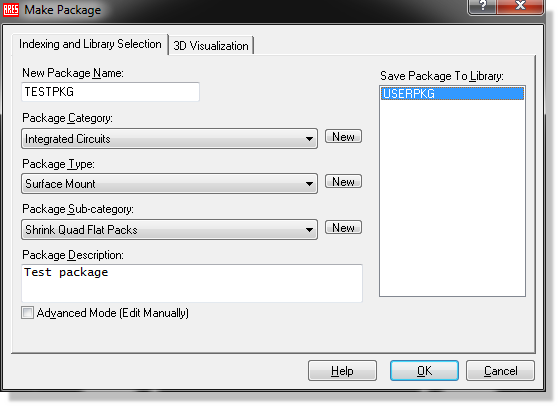
The Make Package dialogue form
You can create your own libraries via the Library Manager – please see the reference manual for details. You should not make your own parts into the other pre-supplied libraries as Labcenter may overwrite these libraries during upgrade installs.
When this is filled out, switch tabs to the 3D Mechanical Model tab (do not hit the OK button at this stage – we still have some work to do). Essentially what we need to do here is provide as much information as possible in order to get a sensible 3D image of the part which can then be used when we use the 3D Viewer to examine a board. This job is greatly aided by a 3D Preview on the dialogue form that will update live as we adjust parameters. Discussion of parameters and values is beyond the scope of this tutorial and is discussed in some depth in the online reference manual (Help Menu Reference Manual). For our purposes, simply fill out the property fields as shown in the next section.
The 3D Mechanical Model Tab
This is where you would either provide a STEP file or use the Labcenter script to provide a geometric model for the part. In either case, you will get a 3D representation of the part in the 3D Viewer and can then export to Solidworks or other MCAD toolchains for case and mounting design.
If you are providing a STEP file you must:
1) Download the STEP file from the internet and place in the MCAD directory of your Proteus installation.
2) Import via this dialogue.
3) Rotate and offset such that the part is aligned correctly on the 2D courtyard. Note that you can zoom in and out on the preview with the middle mouse wheel (or buttons) and the flip command will mirror the board at its current position.
Fortunately, this job is greatly aided by the number of STEP files available on the internet (e.g. www.3dcontentcentral.com) and a 3D preview on the dialogue form to help with alignment.
Setting the 3D parameters
Discussion of geometric model parameters, values and importing models is beyond the scope of this tutorial and is discussed in some depth in the online reference manual (Help Menu – Reference Manual). Geometric models are ideally suited to large pin count parts with small extrusion (e.g BGA, QFP)
STEP files, while common, are often poorly made resulting in large file sizes. Bear in mind the bigger the STEP file the slower the 3D Viewer will render. Consider using geometric models where no sensibly sized STEP file is available.
If you now select the Package Icon, you will see that TESTPKG has appeared in the Object Selector, and can be placed like any of the packages you have used so far. Also, if you place the part on the layout and open the 3D Visualiser from the module toolbar at the top of the application you will see the 3D rendered image of the part.